WaveTrain Adaptive Optics Configuration Guide

This guide complements the basic WaveTrain User Guide. In the present document we discuss the mathematical background and provide usage instructions for a set of Matlab-based procedures whose purpose is to create and analyze adaptive optics (AO) configurations. These AO configuration tools serve the following purposes:

To generate suitably formatted AO input data for WaveTrain simulation runs.
To study AO issues such as wavefront reconstruction, generation of deformable mirror influence functions, and so forth, with or without allied use of WaveTrain.
To assist in analyzing experimental data, either independently or in concert with WaveTrain simulated data.

The AO configuration tools consist principally of Matlab m-files, and are meant to be used from the Matlab command window. The tools contain a number of alternatives for computing the same type of end result. For example, facilities are provided for performing both zonal and modal reconstruction, with a variety of options for each category. The present document will attempt to cover all the significant options included in the AO tools. For historical reasons, the AO tools do not comprise a perfectly integrated set, and they do not present a completely unified user interface. In the present document, we will clarify the principal ways of using the toolset, and the principal alternatives that exist for performing the same functions.

If the user employs the AO tools to provide input to a WaveTrain simulation system, then the tools calculations typically constitute a preprocessing step performed prior to the running of a WaveTrain simulation system. A typical task would be the specification of a wavefront sensor (WFS) and deformable mirror (DM) geometry, and the subsequent computation of DM influence functions and reconstructor matrices. These are all one-time tasks, to be completed prior to the execution of WaveTrain simulation runs. These tasks are setup operations that should be considered part of the complete process of constructing a WaveTrain system and defining its input parameters. The difference is that the AO tools make no use of the TVE (tempus visual editor) environment. The connection between the AO tools functions and the WaveTrain simulation run is that certain data vectors and matrices computed by the AO tools are intended to be read into WaveTrain subsystems via the subsystem input parameter lists. Two key examples are the subsystems HartmannWfsDft and DeformableMirror, which require AO geometry and influence matrix data to do their jobs.

As noted above, the AO tools functions are also useful for various AO analyses independent of any particular WaveTrain simulation. The tools functions can be used to study various mathematical issues related to wavefront reconstruction algorithms, or they can be used to analyze experimental WFS data, entirely within the Matlab environment.

One of the chief restrictions of the AO tools is that the whole set is built around a slope-measuring WFS, such as a Hartmann-Shack sensor. However, the tools interact in such a way that user customization is relatively straightforward.

Table 1 very briefly summarizes the main sequences of AO tools functions available to carry out two principal overall tasks. The most general task is the derivation of a reconstructor matrix to drive the DM actuators for a given WFS-DM geometry. A more restricted task is the derivation of a reconstructed wavefront (WF) when we simply sense the optical field but are not interested in driving a DM. The restricted task differs from the general one in that DM influence functions never enter the picture. The restricted task is not necessarily a simple subset of the general one, because an algorithm that determines DM actuator commands in terms of WFS measurements does not necessarily form an explicit reconstruction of the wavefront as an intermediate step. Table 1 serves as a quick reference guide to the available procedures, which are individually explained in detail as the configuration guide unfolds.

TASK	AO TOOLS FUNCTION SEQUENCE	COMMENTS

WF reconstruction, no DM, zonal	aogeom lsfptos aorecon	(a) Use of lsfptos must be followed (manually) by the correction factor (1/dxyact). (b) aorecon has several options, each leading to a different reconstructor.
WF reconstruction, no DM, modal (Gavrielides)	aogeom slope2mod mod2opd
WF reconstruction, no DM, Southwell	aogeom Documentation of this option is under construction.

Reconstruction with DM, zonal	aogeom aoinf aorecon	A specialty option is the waffle-constrained reconstructor: this substitutes lsfptosw for aoinf.
Reconstruction with DM, modal (Gavrielides)	aogeom slope2mod mod2opd aoinf aorecon

Table 1: Summary of AO tools sequences for major overall tasks

Outputs of the AO configuration tools

As one possible example, consider the sequence of functions aogeom-aoinf-aorecon (see Table 1, task "Reconstruction with DM, zonal)". aogeom is a Matlab-based graphical user interface (GUI) which assists the user in defining the geometry of an AO system that contains a DM and a Hartmann or Shack-Hartmann WFS. Using aogeom, the user defines the geometric layout of DM actuators and WFS subapertures, as well as the shape and extent of the DM actuator influence function. The resulting information is stored in a .mat file for processing by aoinf, a Matlab function which computes the DM optical path difference (OPD) and slope influence function matrices. The output of aoinf is another .mat file, which can then be processed by aorecon, a Matlab function that computes least-squares or "pseudo-inverse" solutions of a matrix system. All the results of this three-step process can be stored to a final .mat file. This composite file can later be used as input to WaveTrain simulation runs, by using the DMModel class constructor in the WaveTrain Runset Editor.

Figure 1: Example of a complete AO system configuration

In the above example, a .mat data file is generated at each major step of the configuration process. This does not necessarily apply to all AO tools procedures. In some cases, one simply generates data vectors or arrays in the Matlab workspace which are passed as inputs to subsequent tools routines. However, the final results of the configuration process, which are needed as input to a WaveTrain simulation system, must always be saved in a .mat file.

An important option to remember is that the final .mat file (the one to be read by the WaveTrain simulation) is allowed to contain any number of reconstructor matrices pertaining to the same AO geometry configuration. For a given AO geometry, it is usually useful to collect in one file several different reconstructor matrices that correspond to different options in the sequence of procedures that yield a reconstructed wavefront or reconstructed DM actuator commands.

Customizing the AO configuration process

It may happen that a user is satisfied with some of the WaveTrain AO tools, but wishes to substitute custom-designed procedures for certain steps. For example, the user may be interested in a special mirror with very specific influence functions, or perhaps a novel reconstruction algorithm. As long as the required variable names and/or .mat files are used and generated by the substitute routines, users can substitute their own computational routines for any or all of the AO tools routines. For example, to do zonal reconstruction with a DM, the tools sequence aogeom-aoinf-aorecon is provided. If desired, a user could replace aogeom with a new Matlab routine that generates the geometry information, and use that routine to generate the .mat input file for aoinf. As another example, a user might be satisfied with aogeom, but might want to replace aoinf with a custom routine to compute influence functions, and finally use the existing aorecon to generate a reconstructor. The fundamental limitations are: (1) to use any of the existing tools procedures, users must interface with them by supplying the expected contents; (2) influence functions and reconstructors must be implemented as matrix multiplications; (3) the custom user routines must of course be consistent with any specific assumptions or limitations in any AO tools routines that are used.

Most generally, a user could perform all AO configuration steps in custom fashion, and simply supply a final .mat file for reading by the WaveTrain runset. The format of all the possible variables that could be used by WaveTrain library subsystems is summarized in the section .mat Interface File Contents.

Setting the Matlab Path

The WaveTrain AO configuration utilities are based in Matlab. Before they can be used, the following directories must be in the Matlab path:

%WT_DIR%\mfiles\aogeom.tbx (the main aogeom routines)
%WT_DIR%\mfiles\aocomp.tbx (the remaining computational routines)

where %WT_DIR% specifies the top-level directory in which WaveTrain is stored. For version 2000.11 %WT_DIR% is usually c:\Program Files\mza\wavetrain\v2007a. The Matlab path can be set using the path command in Matlab or the Set Path utility (accessed from the File menu). See Matlab documentation for more information.

When the above two directories have been added to the Matlab path, the AO tools routines can be invoked from any working directory.

Coordinate Systems

In WaveTrain, all input and output quantities are consistently expressed in MKS units. In particular, all distances are expressed in meters. This convention applies to all the AO tools functions as well. In particular, wavefront OPD values and DM actuator displacements will be expressed in meters, and wavefront slopes will be expressed in radians of tilt angle.

WFS/DM space and object space

When modeling AO components (wavefront sensors, deformable mirrors, or beam steering mirrors), the most common wave-optics modeling practice is to project the adaptive-optics geometry parameters to object space (i.e., beam dimensions outside the telescope). Using this approach, the AO component parameters can be easily related to the turbulence parameters of the propagation medium. For example, the WFS subaperture and DM actuator spacings are specified according the dimensions of their images in the entrance pupil of the telescope system. In connection with this procedure, it is important to note that, in constructing a WaveTrain system, we usually place all the optical system components in the same plane (the entrance pupil), with no physical propagation distance between any of the components. Of course, the order of operations carried out by various elements (e.g., splitting, attenuating, tilting, sensing, etc.) corresponds to the order in which the WaveTrain blocks are connected, and this can be made consistent with their actual positions in the physical system. In most WaveTrain modeling, there is no reason to carry out physical-optics propagation using Fresnel propagators within the optical system. The one usual exception to this is the far-field image in (or near) a focal plane. The diffractive effects of the entrance pupil are accounted for by propagations embedded in WaveTrain's camera or wavefront sensor modules. Defocused sensor planes can be accounted for as well in this framework. The omission of diffractive propagation between most elements of the optical system is consistent with the usual optical analysis of composite systems: the effects of diffraction are for practical purposes completely represented by one physical propagation from pupil to sensor plane.

When using this projection modeling approach for the AO elements, users must ensure that the proper scaling and magnification is configured within the simulation. In particular, the specifications of WaveTrain sensor subsystems must be scaled to correspond to their projected dimensions.

Relations among WaveTrain propagation and AO meshes

As explained in the basic WaveTrain User Guide, WaveTrain's propagation mesh (the mesh on which the Fresnel propagations are performed) is determined by the location of sensors relative to sources. The propagation mesh is always centered on the local (x,y) origin of the pupil of a sensor module, and this applies to wavefront sensors as well. When specifying (x,y) coordinates for subapertures and actuators (using the aogeom tool), these coordinates should be interpreted as local coordinates relative to the pupil of the wavefront sensor or AO subsystem in question. This applies in particular if the WaveTrain system contains more than one wavefront sensor or AO subsystem that are displaced from each other using TransverseVelocity (displacement) blocks. This convention allows easy reuse of the AO coordinate specifications in a multi-aperture system that has AO subsystems behind each aperture.

In the AO configuration tools, three new meshes are defined. The points of these meshes correspond to WFS subaperture center positions, DM actuator positions, and points at which a wavefront OPD is to be evaluated. The AO tools allow considerable freedom in specifying the relative location of the mesh points, although there are certain constraints that may depend on the tools function in question. Whatever the exact specification method may be, the AO meshes are all referenced by means of specified offsets relative the local (x,y) origin. A WaveTrain simulation system will mate the AO setup information to the propagated wave by applying the necessary interpolation procedures. As one example, consider the size of a typical WFS subaperture compared to the propagation mesh. Given the practical constraints on propagation mesh point dimension, there will likely be very few propagation mesh points across one subaperture, and furthermore, the spacing may not be "nicely" related to the subaperture spacing. In order to adequately compute the spot shape in the WFS focal (sensor) plane, WaveTrain's HartmannWfsDft module will interpolate the incident optical field (which is defined on the propagation mesh) onto a mesh used for computing the Fourier Transforms that HartmannWfsDft performs for each subaperture. As a second example, consider the effect of a DM on an incident wavefront. The instantaneous deformation of the DM is defined on a mesh specified by the AO configuration tools, which is not required to have any exact relation to the propagation mesh. But of course, when WaveTrain applies the DM correction to the wavefront, it must do so on the propagation mesh, in preparation for a subsequent physical propagation operation. In this situation, WaveTrain also automatically performs the necessary interpolation.

Overall rescaling of an AO configuration

Setting up a particular combination of AO geometry, influence function, and reconstructor is a fairly elaborate procedure. It may occur that one wants to rescale a given configuration to a different telescope aperture size. This arises in practice since one may have a given (expensive) DM that one wishes to use with various telescope apertures. WaveTrain provides a rescaling argument in the DMModel function, which allows the AO configuration results to be rescaled to a different aperture size without redoing the configuration procedures.

Background: AO Geometry, Influence Functions and Reconstructors

In this section, we review the mathematical operations performed by WaveTrain's AO configuration tools. These tools consist principally of Matlab m-files, and are meant to be used from the Matlab command window. A small number of the tools can also be executed from the operating system console window. In general, the AO tools facilitate the specification of a certain class of AO geometries, and provide various options for wavefront reconstruction and the generation of DM actuator commands. The tools routines are structured in such a way that the user may replace individual elements by user-supplied routines.

The present section of the AO Guide has two goals:
(1) We provide sufficient conceptual background material to clearly specify just what quantities one can set up and compute using the AO configuration toolset.
(2) We identify the principal Matlab routines that are provided to compute the AO setup quantities. The principal routines work together in groups as indicated in the cells of Table 1.

Later sections of the AO Guide, entitled "Matlab function details: XXX", describe in further detail the GUI windows and the exact syntax of all the Matlab routines.

Actuator-subaperture geometry

The aogeom tool facilitates the specification of rectangular (in fact, mostly square) meshes of WFS subapertures and DM actuators. Regions of active, slave and inert actuators are then defined by circles of various radii. The routine aogeom differs from all the other AO tools in this sense: by running aogeom, the user starts and then interacts with a graphical user interface (GUI). All other routines discussed in this guide are ordinary functions that take input arguments from and return output arguments to the Matlab workspace.

WFS and DM alignment is specified with respect to the local coordinate origins of the wavefront sensor or AO subsystems. In aogeom, the alignment is specified by an (x,y) offset for the subaperture mesh and another offset for the actuator mesh. If these offsets are both (0,0), then the meshes are registered in the so-called Fried geometry, wherein the actuators lie at the corners of the subapertures. Figure 3 illustrates the Fried geometry. Positioning the actuators at the subaperture corners allows the best match between DM deformation and subaperture WF slopes, and minimizes potential problems with unsensed wavefront modes. Equal but non-zero offsets would still preserve the Fried geometry, but would offset the center of both meshes from the center of the propagation mesh. An equal-offset specification is allowed, although it usually serves no purpose.

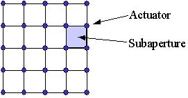
Figure 3: The Fried geometry (perfectly registered meshes)

Using aogeom, one may also create departures from the Fried geometry, by making the actuator mesh offset different from the subaperture mesh offset. This is considered "misregistration" of the meshes. Of course this can occur in practice, and it may be important to simulate and study the resulting performance effects.

CAUTION: Before attempting to set up a misregistered system, the user should study the Guide section Working with Asymmetric and/or Misregistered Systems. Note in particular that the aoinf routine for computing influence functions does not work if there are departures from the Fried geometry. In addition to a shift misregistration, aogeom also allows another form of misregistration, namely an actuator spacing not equal to the subaperture spacing. This could arise in a physical system due to imperfect magnification match between the WFS and DM paths.

aogeom by itself does not perform any calculations that depend on the fill factor of the subapertures. As will appear in the GUI discussion below, the only subaperture size specification in aogeom is the "subaperture spacing" (i.e., center-to-center spacing). The implicit assumption is that the subapertures are square, with a 100% fill factor, which is typical for Hartmann-Shack lenslet arrays. But this assumption is only used when WaveTrain's HartmannWfsDft subsystem segments an incident beam and computes the sensor-plane irradiance formed by each subaperture. A WaveTrain system can model a more general fill factor, but to do so the user must create and insert a transmittance mask in the WaveTrain system in front of HartmannWfsDft. The mask can be created by using WaveTrain's Apodizer system. If a transmittance mask is added, the use of aogeom is unchanged.

Geometry specification when no DM is present

If we are interested solely in computing a reconstructed wavefront, with no DM and no correction loop in mind, then we still use aogeom to define the WFS subaperture geometry. Furthermore, defining "actuator" positions in aogeom can also still be useful, even though no DM will be present. Given "actuator" position specifications, aogeom simply creates vectors that list the "actuator" x and y coordinates in a special ordering scheme. Then later, when using some of the routines that produce reconstructed WF values, the so-called "actuator" position vectors can be used to specify the points at which one desires the evaluation of the reconstructed WF.

Vector representation of subaperture, actuator, and wavefront meshes

In the AO tools, the coordinates of subaperture centers, actuators, and points where wavefronts are evaluated or reconstructed are represented by 1-D vectors, where the 2-D (x,y) layout of the mesh points is organized for algorithm convenience into a 1-D vector. This is a convenient format for matrix representation of the algebra, but the main motivation for the 1-D representation is generality: subaperture (and mirror actuator) locations can have a rather arbitrary layout, with complications such as annular holes, irregular borders, rectangular or hexagonal meshes, and so forth. Not all of these features are presently available in the AO tools, but to include them in the future (or now by user customization), the 1-D representation is the best approach.

Thus, we have the following vectors:

xsub = a column vector of dim (n_sub x1), containing the x-coordinates of the centers of the WFS subapertures. The subaperture indexing (ordering) convention will be described later.

ysub = a column vector of dim (n_sub x1), containing the y-coordinates of the centers of the WFS subapertures.

xact = a column vector of dim (n_act x1), containing the x-coordinates of the actuator locations. The actuator indexing (ordering) convention will be described later.

yact = a column vector of dim (n_act x1), containing the y-coordinates of the actuator locations.

These four data vectors (and the length scalars nsub and nact) appear as variables in the .mat file created by aogeom. As noted previously, all distances in AO tools (including OPDs), and in WaveTrain generally, are expressed in meters.

Similarly, in our AO background discussion, we will use the following vectors:

s = column vector of subaperture slopes, dim (2n_subx 1)
= [s_x(r₁) ,..., s_x(r_nsub), s_y(r₁), ..., s_y(r_nsub)]^T , in units of radians of angle.
Note that:
(a) the ordering 1,...,n_sub is the same as the xsub and ysub vectors;
(b) the x and y slope components have been concatenated into one vector.

d_act = vector of actuator displacements, in m; dim (n_actx 1).
The ordering is the same as the xact and yact vectors.

d_opd = vector of wavefront surface displacements, in m; dim (n_opdx 1).
The displacements are defined with respect to a flat, 0-tilt reference wavefront.
n_opd may be identical to n_act (see, e.g., routine lsfptos), but may also represent a denser mesh.

The notation d_opd to characterize the wavefront implies that a continuous surface of constant phase exists, so that a DM with a continuous facesheet can be shaped to compensate. The extent to which this is valid depends on the integrated strength of turbulence, but the reconstruction procedures included in the AO tools are based on this concept.

Note that in the WaveTrain propagation code, the 1-D representation of DM displacements is eventually converted to a 2-D array representing the corresponding phasor exp[i*(2p/l)*d(x_i,y_j)]. The correction applied to an incident wavefront is then based on manipulation of the 2-D complex-field arrays.

Subaperture slopes, reconstructed wavefronts and DM actuator commands

The AO tools emphasize a slope-measuring WFS with discrete subapertures, such as a Hartmann-Shack device. Since the basic data consists of a set of discrete slopes, s_data, the tools functions are mainly oriented toward producing a (linear) mapping that directly converts s_data into either a reconstructed WF d_opd , or into DM actuator commands d_act . In either case, the net linear mapping will always be represented as a 2-D "reconstructor" matrix, generically denoted by R, connecting the 1-D vectors in question:

d_{opd, rec} = R s_data , or dd_act,rec = R s_data .

Regardless of the details of the reconstruction method, and of any complications due to DM faceplate influence functions, final results will always be expressed in this common format. The reconstructor Rremains fixed, for a given WFS geometry, as the incident wavefront fluctuates in a dynamic system. One or more R matrices are key components of the final .mat file that must be produced by the AO tools to configure a WaveTrain simulation that uses a DM.

In the following sections, we present several different reconstruction methods, each of which may have a number of sub-options. In the final .mat output file created by the use the AO tools, the user may store more than one reconstructor matrix for a given WFS/DM geometry. Later, the WaveTrain simulation can read whichever reconstructor variable name is desired for a particular simulation run. If desired, the WaveTrain system could also split light among parallel paths, thus allowing a comparison of several reconstruction algorithms within one system and run .

Reconstruction of a wavefront (no DM) from subaperture slopes

The goal here is to develop a reconstructor mapping that directly converts s_data into a reconstructed wavefront opd vector d_opd : d_opd,rec = R s_data . The displacements d_opd are defined with respect to a flat, 0-tilt reference wavefront. The following sections explain alternate approaches for which code modules exist in the AO tools.

Zonal reconstructor for wavefront

To perform a zonal WF reconstruction using the WaveTrain AO tools, the approach is to sequentially execute the functions aogeom, lsfptos, and aorecon. aogeom is used to establish the geometry of subapertures and their corner "actuator" positions, as introduced previously. In the present context, the significance of the so-called "actuator" positions is simply that they define mesh points at which the WF phase will be computed. We regret the somewhat confusing dual-use terminology.

In the present reconstruction calculation, misregistration is not allowed: the "actuators" in aogeom must be placed at the subaperture corners, or the subsequent calculation using lsfptos makes no sense. Also, there is no significance to slave actuators in this situation: all the actuators should be designated as masters in preparation for using the lsfptos function.

Using the geometry information, the function lsfptos carries out the following calculation. Consider one subaperture, as illustrated in Figure 5. The labels c_i denote the subaperture corners. The d_opd,i denote the WF displacements at the corners, with respect to a 0-tilt plane wave across the entire complex of subapertures. One can approximate the average surface slopes of this WF patch by simple bilinear interpolation, namely

s_x = 0.5 * [(d_opd,2 -d_opd,1)/dx + (d_opd,4- d_opd,3)/dx]
s_y = 0.5 * [(d_opd,3 -d_opd,1)/dy + (d_opd,4 - d_opd,2)/dy]

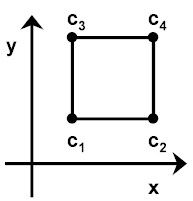
Figure 5: A single subaperture in a Fried geometry

For the whole set of subapertures, one can use these equations and adjacency information to create the matrix relation

s = S'_cd_opd,c , where matrix S'_c has dims (2n_sub x n_opd,c).

We use the subscript "opd,c" to emphasize the fact that n_opd,c is the number of subaperture corner points. Note that in the present procedure, the opd mesh has the same spacing as the subaperture mesh (though offset to the corners). In some later procedures involving DM influence functions, we will introduce opd meshes that are denser than the subaperture mesh. The Matlab routine lsfptos provided with the AO tools computes S'_c , assuming that d_opd,c is in meters, and s is in radians of angle.

CAUTION: the routine lsfptos actually omits the (1/dx,dy) factors, which must be appended manually to obtain the correctly-scaled slope angles in radians of angle.

Now, if we have WFS slope data, s_data, then we can obtain a "reconstructed" WF, d_opd,c;rec , by solving the equation s_data = S'_cd_opd,c in a least-squares sense. A least-squares (or some analogous) approach is necessary since S'_chas more rows than columns (there are more equations than unknowns). The AO tools provide several elaborations on the classical least-squares solution, so we will use the term "pseudo-inverse" to generically designate the solution:

s_data = S'_cd_opd,c ==> d_opd,c;rec = (S'_c)^# s_data

= R'_c s_data

We use the superscript notation (...)^# to indicate the "pseudo-inverse". More generally, we will use the notation R to represent a reconstructor matrix (a matrix that transforms a slope data vector into wavefront opd or into actuator commands, as the case may be). Note that the reconstructor (S'_c)^#remains fixed, for a given WFS geometry, as the incident wavefront changes in a dynamic system. The AO tools provide the function aorecon to compute the pseudo-inverse of any specified matrix.

In sum, to perform a zonal WF reconstruction, we require the tools functions aogeom (define subaperture geometry), lsfptos (compute S'_c matrix), and aorecon (compute pseudo-inverse (S'_c)^#). Full details of the available options, and examples of Matlab terminal sessions, are given in later sections devoted to lsfptos and aorecon. Background information regarding one key option of aorecon, namely the singular-value decomposition, is discussed next.

Least-squares solution and singular-value decomposition

Given any overdetermined matrix system (more rows than columns) written as

s = S d,

the classical least-squares solution, derived in numerous textbooks, can be shown to be equivalent to solving the matrix equation

S^Ts = S^TS d, where T=transpose, and (S^TS) is a square matrix, presumed to be of full rank.

Assuming (S^TS) is not exactly singular, the classical solution can now be written in the matrix form

d_rec = (S^TS)^-1S^Ts = R_clas s , where (.)^-1 designates a true inverse.

We use the symbol R in general to denote a "reconstructor" matrix that maps a given s to the "reconstructed" d_rec, and R_clas stands for the classical least-squares solution (S^TS)^-1S^T.

Although the square matrix (S^TS) is usually not exactly singular, so that a numerical inverse does exist, it turns out in practice that (S^TS) often has a very high condition number. This is equivalent to saying that the matrix is in a certain sense "close" to singular, or that the solution R_clas can produce results with poor numerical stability. Poor stability in this context means that small changes in the data s(due, e.g., to measurement noise) produce large changes in d_rec. In practice, this can introduce meaningless solution jumps and stability problems with the control system. Modern numerical analysis has developed a method of solving the least-squares problem that allows one to identify and eliminate "modes" which are associated with the numerical instability. This method is based on a matrix factorization of rectangular matrices called the singular-value decomposition (SVD). The AO tools function aorecon allows the user to first compute the SVD, and then to compute the reconstructor matrix R after specifying which modes to remove. This requires executing aorecon twice, with two different sets of arguments. If no modes are removed, the solution reduces to the classical R_clas. The later section on aorecon illustrates the Matlab syntax details and usage options.

The SVD option of aorecon can be used regardless of the precise context in which aorecon is used. Note that removing the near-singular modes is often critical to the construction of a stable least-squares solution.

REFERENCES:

(1) G.E. Forsythe, M.A. Malcolm, and C.B. Moler, Computer Methods for Mathematical Computations, chs. 3 and 9, Prentice-Hall, 1977.
(2) G. Strang, Linear Algebra and its Applications, 2nd ed., Academic Press, 1980.
(3) Golub and VanLoan, Matrix Computations, Chs. 2 and 6, Johns Hopkins U. Press, 1983.

Modal reconstructor for wavefront

To perform a modal WF reconstruction using the WaveTrain AO tools, the approach is to sequentially execute the functions aogeom, slope2mod, and mod2opd. aogeom is used to establish the geometry of the subapertures, as introduced previously. Even though no DM is present, the corner "actuator" positions in aogeom may be used later to define the points at which the WF phase will be reconstructed; however, the modal reconstructor can directly yield the reconstructed WF at other points as well.

The previous section explained "zonal" reconstruction: in that procedure, samples of wavefront opd were defined at the corners of every subaperture "zone", and these samples were considered independent variables on an equal footing, to be solved for via a least-squares fit. A strong point of the zonal procedure is that it works easily with any WFS geometry. In particular, the algorithm for computing the S'_c influence matrix is the same whether or not there is a central obscuration, or an irregular boundary. The only thing that is needed is the identification of each subaperture with the corner points that surround it.

An alternate reconstruction procedure, known as "modal reconstruction", begins by expressing the wavefront opd as a superposition of some convenient set of mathematical basis functions ("modes"). In this case, the expansion coefficients become the unknown elements to be reconstructed, after truncating the sum at some finite order. The elements to be solved for do not directly represent local ("zonal") displacements, but rather the modal amplitudes.

A feature of modal reconstruction is that it inherently contains an extra degree of freedom relative to the zonal reconstructor, namely the number of modes for which the user wants to solve. Modal reconstruction has several purposes:

There is important theoretical work on AO correction that is based on modal decomposition of the wavefront. Thus, using a modal reconstructor with data allows one to make close contact with this theory.
One may wish to implement an AO system that only corrects a selected set of modes. This may be desired for various reasons: (a) complexity or cost limitations, (b) use of more than one corrector element with different properties for different modes, (c) use of post-processing to correct higher-order aberrations, (d) experimental situations (e.g., thermal blooming) where one wishes to ignore certain modes because of special control instabilities that can arise.
The subtleties of numerical conditioning (solution stability) may play out differently in the inversions associated with modal and zonal expansions.

A disadvantage of modal reconstruction is that it is more difficult to treat general WFS geometries. There are several related complications, but the basic problem is that one wants to use basis functions that are orthogonal on the support of the optical pupil. Therefore, different geometries require algorithm development with different basis sets. The modal routines presently available in the AO tools allow the modeling of unobstructed circular and annular pupils, via the Zernike circle polynomials and Zernike annular polynomials, respectively.

Consider the following expansion of the wavefront opd:
d_opd(r) = S_{k=1...nmod} a_k Z_k(r)

where the Z_k are the basis functions, a_k are the expansion coefficients, nmod modes have been retained, and r is an arbitrary position. The AO tools implement a procedure in which the Z_k basis is the Zernike circle or annular polynomial set. For a discrete set of sample points {r_i}, we express the preceding equation in matrix form as

d_opd = Z a_mod

where Z_i,k = Z_k(r_i) , a_mod = [a₁,...,a_nmod ]^T, and d_opd = [d_opd(r₁),...,d_opd(r_Nopd)]^T .

The goal of the modal reconstruction is to estimate a_mod , and finally d_opd, from s_data. The AO tools implement a procedure developed by Gavrielides. The key concepts are as follows:
(1) In continuum space, the wavefront slope is the gradient of d_opd(r):
s(r) = grad{d_opd(r)} = S_{k=1...nmod} a_k grad{Z_k(r)}

(2) Therefore, if we had a set of two-vector functions that were orthogonal to the gradient of the Zernikes, we could immediately apply a projection integral to the preceding equation to solve analytically for any a_k.
(3) Gavrielides derived a set of vector polynomials that satisfy (2).

(4) By discretizing the projection integral on the subaperture mesh, we obtain the matrix formulas

a_{mod, rec} = V s_data , and therefore

d_{opd, rec} = Z a_{mod, rec}= Z V s_data = R_mod s_data .

The notation R_mod = ZV defines the final reconstructor matrix that converts a slope data vector into a wavefront opd.

After aogeom is used to define the geometry of the subapertures, the AO tools provide two further functions that implement the modal reconstruction described above: function slope2mod computes the V matrix for a specified WFS geometry, and function mod2opd computes the Z matrix for a specified opd mesh. Syntax details of slope2mod and mod2opd are given in a later section.

Notice that this reconstruction method does not require a least-squares solution to obtain the wavefront. However, when we later extend the procedure to the computation of DM actuator commands that will correct the perturbed wavefront, we will see that a least-squares solution does enter.

REFERENCES:

A. Gavrielides, "Vector polynomials orthogonal to the gradient of Zernike polynomials", Optics Letters, Vol. 7, No. 11, November 1982, pp. 526-528.

Zonal 2 (Southwell) reconstructor for wavefront

An alternate method of zonal WF reconstruction is due to Southwell. To perform the Southwell reconstruction using the WaveTrain AO tools, the approach is to sequentially execute the functions aogeom, ...

This section is under construction.
REFERENCES:

Southwell, " "

Reconstruction of DM actuator commands from subaperture slopes

This task differs from the underlying reconstruction of a wavefront in two ways:
(1) we have the extra complication of DM facesheet influence functions;
(2) in closed-loop operation with a DM, the WFS slopes represent the difference ("error") between the mirror shape and the wavefront. We now want to develop a reconstructor mapping that directly converts s_data into the actuator displacements dd_act required to null the residual WF perturbation: dd_act,rec = R s_data . For closed-loop operation with a DM, we use the notation dd to emphasize the fact that, at any time instant, the WFS slopes represent the difference between the mirror shape and the wavefront, so that dd_act,recrepresents the change that needs to made to the current actuator displacements. The new commands to be specified to the mirror would be d_act,new = d_act,old + dd_act,rec.

Deformable mirror influence functions (OPD and slope)

A continuous DM facesheet has some stiffness, so that pushing or pulling the facesheet with a point-like actuator tip may cause facesheet displacement at significant distance from that actuator, with a particular deformation shape. Provided that the mirror is operating in a regime where the superposition principle applies, the net deformation can be expressed as the sum of the deformations due to the individual actuators. The deformations at a set of discrete points can then be expressed in terms of the actuator displacements by means of a matrix multiplication. In the AO tools, this matrix is called the "OPD influence function", although we should bear in mind that the matrix yields the surface displacements.

We use the notation

        d_act = vector of actuator displacements, dim (n_actx 1), in units of m
        d_srf   = vector of mirror surface displacements, dim (n_opdx 1), in units of m.
                    We express the dimension of d_srf as n_opd because at each surface point we
                    can compute the resulting opd correction to the incident wavefront. The AO
                    tools allow this opd mesh to be specified with a density higher than the actuator
                    or subaperture mesh.

The DM OPD influence matrix is defined by the relation

        d_srf = Ad_act ,   where the OPD influence matrix, A, has dims (n_opdx n_act).
                                  Depending on how well one wishes to resolve the DM surface shape,
                                  the dimension n_opd may be very large. However, the number of surface
                                  elements affected by a given actuator is usually small compared to n_opd.
                                  That is, most elements of A are 0, and A can be stored in a sparse format.

When the DM is used at near-normal incidence (the usual practice), the DM surface deformation produces an opd change in the (already perturbed) incident wavefront of

dd_opd = 2d_srf= 2Ad_act .

Now, in closed-loop operation, the WFS slopes represent the difference between the current mirror shape and the wavefront. If we denote this difference as dd_opd, then we can write

s = S'dd_opd , where matrix S' has dims (2n_sub x n_opd).

The matrix S' could be taken as the S'_c matrix that we defined for zonal wavefront reconstruction, if we define the opd mesh to be exactly the actuator mesh. However, for generality, we allow the opd mesh to be denser. Combining the previous equations yields

        s = 2S'A dd_act
           = S dd_act ,   where matrix S has dims (2n_sub x n_act), and where dd_act denotes the
                                extra actuator displacements required to null the current slopes.

Any matrix S that takes actuator displacements into slopes is called a DM slope influence matrix.

The AO tools function aoinf computes linked DM opd and slope influence matrices. A complication that arises in practical DM systems is that we do not necessarily treat all actuators on an equal footing. As discussed in connection with aogeom, we may classify actuators as either masters or slaves. In that case, the DM slope influence matrix, S, must be further refined. The aoinf function includes this refinement if the geometry setup has specified a non-zero number of slaves. The zonal reconstructor discussed next allows for this refinement. Note that the master-slave distinction has no impact on the DM opd influence function, A: the A matrix operates on all the actuators, and has the same values regardless of slaving identifications.

Choice of influence function shape

The values of the A matrix computed by aoinf depend on the specification of an analytic model for the facesheet deformation due to a point force. The WaveTrain AO tools provide five choices of influence function shape for the OPD influence function. Since the shape is considered geometry information, the specification of shape is done in the aogeom GUI. The shape choices are denoted as Green's Function, Gaussian, Piston, Linear, and Cubic. For a given shape category, the user also specifies width parameters. Details are given in the AO Geometry Parameters section, in the subsection Influence Function Entries. Given a choice of shape and width parameters, the subsequent execution of aoinf generates the corresponding DM OPD and slope influence matrices.

Zonal reconstructor for DM actuator commands

To obtain DM actuator commands using a zonal reconstruction, we will require the AO tools functions aogeom, aoinf, and aorecon. aogeom is used to establish the geometry of subapertures and their corner actuator positions, as introduced previously.

In the previous section on DM influence functions, we obtained a matrix S defined by

s = S dd_act , where matrix S has dims (2n_sub x n_act).

Given S and some WFS data s_data, we must solve the preceding equation for the dd_act.to find the additional mirror deformation required to null the current error. The solution requires a least-squares or "pseudo-inversion" approach, since S has more rows than columns. Using the superscript notation (...)^# to indicate a pseudo-inverse operation, we write formally

dd_act = S^# s_data = R_zon s_data ,

defining the zonal reconstructor matrix R_zon = S^#. The AO tools function aorecon is provided to compute the pseudo-inverse of any specified matrix. Details of the available options, and examples of Matlab terminal sessions, are given in the later section devoted to aorecon. One of the key options of aorecon is the capability to perform singular value decomposition.

Refinement of the influence function: master and slave actuators, and actuator voltages

The above paragraphs define the zonal reconstruction concept, but when using the AO tools functions the user must be aware of several complications and refinements. These refinements do not require extra steps on the user's part, but they introduce extra terminology and variables which may initially cause some confusion. In future releases, we plan to clean up and streamline the present procedure.

Frequently, the actuators of a DM are not all treated on equal footing, in the following sense. As discussed in further detail in the geometry section, active (i.e., non-inert) actuators are divided into the categories of "masters" and "slaves". The displacement of a slave actuator is constrained to be a fixed linear combination of a few neighboring master displacements. If we have slaves in the DM configuration, then in order to guarantee the desired slaving relations, the slope influence function should be modified to automatically incorporate the slaving constraints. The result is a modified influence function that maps a vector of only master actuators to all the subaperture slopes. This modified influence function, rather than the full S, is the quantity that will be pseudo-inverted to form the reconstructor.

A final complication that is allowed for by the AO tools concerns a conversion between actuator displacements and actuator voltages. The voltages are the physical input quantities provided to a DM by a physical hardware control loop. The motivation for modeling this extra degree of freedom was not to represent a simple proportionality factor between applied voltage and displacement. The original motivation was to model cross-talk that existed with a specific DM that was of interest during early stages of WaveTrain development. The original motivation is no longer relevant, and in contemporary work with WaveTrain, the voltage-to-actuator displacement matrix is by default the diagonal unit matrix. The only reason for discussing this here is that, when working with some of the AO tools functions, the user must deal with variable names that reflect this early side-track in development.

The refinements discussed in the preceding two paragraphs are expressed quantitatively by the chain of linear mappings dd_act <== dv_act <== dv_mas , where dd_act is the vector of all actuator displacements, dv_act is the vector of all actuator voltages, and dv_mas is the vector of master actuator voltages. Therefore, the original formulation of the slope influence function, s =S dd_act , becomes

        s = S dd_act
           = S * (vtod) * (mvtov) * dv_mas
           = (mvtos) * dv_mas   ,

where we have introduced notation of programming-variable style:
         (mvtov) = matrix that maps master-actuator volts to all-actuator volts (dims n_act x n_mas)
         (vtod)    = matrix that maps all-actuator volts to all-actuator displacements (dims n_act x n_act)
         (mvtos) = matrix that maps master-actuator volts to all subaperture slopes (dims 2n_sub x n_mas)

The matrix names written in programming style are actual variable names generated in the Matlab workspace when using the AO tools functions. A full list of variable names is given in a later reference section.

The key points for the AO tools user are:
(1) The composite matrix (mvtos) is automatically computed by running the function aoinf. An example of the Matlab command sequence is given in the section where syntax details of aoinf are specified.
(2) The composite matrix (mvtos) is the input variable that must be pseudo-inverted when using the aorecon function to finally compute the reconstructor. This holds even if no slave actuators have been defined in the geometry.
(3) The OPD influence matrix generated by aoinf, denoted A in our theoretical development, has the Matlab variable name (opdif).

In sum, zonal reconstruction of DM actuator commands requires the use of tools functions aogeom (define geometry), aoinf (compute A and mvtos), and aorecon (compute pseudo-inverse of mvtos).

Tilt removal option

In AO systems that contain both a fast-steering mirror and a WFS, some undesirable coupling may occur if both elements are trying to correct residual tilt. Therefore, an important option provided by routine aorecon is the computation of tilt-included or tilt-removed reconstructors. "Tilt-included" signifies that the reconstructor will generate an estimate of the complete wavefront impinging on the WFS, whereas "tilt-removed" signifies that the full-aperture tilt term is projected out of the reconstructed wavefront. The tilt-removal option is independent of the SVD option.

Waffle-mode removal option

The Fried geometry of subaperture-actuator placement is susceptible to the appearance of a particular unsensed DM mode called "waffle". This consists of a saddle-like deformation of the surface patch corresponding to any subaperture, where the two actuators on one diagonal are equally high, and the two actuators on the other diagonal are equally low. The pattern is illustrated in Figure 6 over a neighborhood of 3 x 3 subapertures. Due to the symmetry, this produces WFS focal-plane spots whose centroid is undisturbed relative to the spots of a flat wavefront: hence, we have an "unsensed mode". Higher moments of the spot shape are affected, but the centroid is not sensitive to those moments.

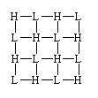
Figure 6: "Waffle" surface deformation in the Fried geometry. H and L mark actuator locations, where H represents a high actuator and L represents a low actuator. The squares define the subaperture areas.

The Wavetrain AO tools offer a reconstructor option that attempts to explicitly remove the waffle component from the actuator command vector. The so-called waffle-constrained reconstructor is a zonal reconstruction method for actuator commands that uses the sequence of AO tools functions aogeom (define geometry), lsfptosw (compute a slope and waffle influence matrix), and aorecon (compute pseudo-inverse). As its name implies, lsfptosw computes a slope influence matrix using the same meshes and a procedure closely related to the previously discussed lsfptos method. Subsequently, the aorecon function is used in the same way(s) as in previously discussed zonal reconstructions. The function details section includes a sample Matlab terminal session that illustrates a reconstructor calculation using lsfptosw.

Depending on the problem details, the explicit removal of waffle implemented via lsfptosw may be redundant. The use of the SVD capability of aorecon may be sufficient to remove any significant waffle component. Nevertheless, the lsfptosw option is provided in the AO tools, so users may experiment on their own particular problems.

REFERENCES:

R.W Praus, II: "Derivation of a Waffle-Constrained Reconstructor (WCR)", Technical Memorandum, MZA Associates Corp., Sep. 1999.

Modal reconstructor for DM actuator commands

To obtain DM actuator commands using a modal reconstruction, we will require the AO tools functions aogeom, slope2mod, mod2opd, aoinf, and aorecon. As usual, we start with aogeom to define the geometry of the subapertures.

In the section on modal reconstruction of wavefronts without a DM, we developed the reconstructor

d_{opd, rec} = Z a_{mod, rec}= Z V s_data .

As discussed previously, the tools functions slope2mod and mod2opd are used to compute V and Z. Now, in closed loop operation with a DM, the WFS slopes represent the difference between the current mirror shape and the wavefront. If we denote this difference as dd_opd, then we can write

dd_{opd,
rec} = Z V s_data .

Without a DM, the ZV product gave the final WF reconstructor. But, to drive the DM, we must compute the corresponding actuator displacements. In terms of the DM opd influence matrix, we have

dd_opd = 2A dd_act , where A has dims (n_opd x n_act), and the opd mesh must of course
be whatever was used to compute Z and V.

As noted previously, the tools function aoinf computes (among other things) the matrix A.

Now, given A, we must solve the preceding equation for the dd_act. To do so requires a least-squares or "pseudo-inversion" approach, since A has more rows than columns. Using the superscript notation (...)^# to indicate a pseudo-inverse operation, we write formally

dd_act,rec = (1/2)A^#dd_opd = (1/2)A^#Z V s_data

= R_mod s_data ,

where R_mod= (1/2)A^#Z V defines the final modal reconstructor matrix, for reconstruction of the DM actuator commands from the WFS slopes.

The AO tools function aorecon is provided to compute the pseudo-inverse of any specified matrix. Details of the available options, and examples of Matlab terminal sessions, are given in the later section devoted to aorecon. One of the key options of aorecon is the capability to perform singular value decomposition.

In sum, modal reconstruction of DM actuator commands requires the use of tools functions aogeom (define geometry), slope2mod (compute V), mod2opd (compute Z), aoinf (compute A), and aorecon (compute pseudo-inverse A^#).

Matlab Function Details: Defining AO Geometry

aogeom - Overview

To start the aogeom GUI enter the Matlab command:

» aogeom

This command brings up a figure window containing a diagram of a default AO system:
(NOTE: it may be necessary for the user to enlarge the default window (using the mouse) to avoid clipping the axis labels)

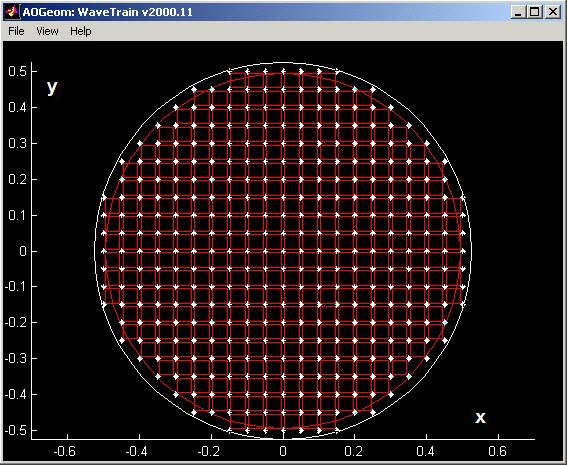
The default AO system is a 21x21actuator mesh designed for an unobscured aperture of 1-meter diameter. The following bullets list the graphical components of the above diagram, and specify the coordinate system:

The white diamonds are master actuators as superposed on the deformable mirror.
The red squares represent the areas of wavefront sensor subapertures, usually configured so the corners fall on actuators.
The white circle shows the outer radius of master actuators.
The red circle shows the outer radius of subapertures. The circle goes through some of the red squares, because the option is selected which keeps any subaperture whose area falls mostly inside the outer subaperture radius.
The axes show the coordinates of the actuators and subapertures, in units of meters. The horizontal axis in the AOGeom window is the x-axis, and the vertical axis is the y-axis.
In WaveTrain these coordinates are usually, but not necessarily, defined in "object space" (i.e., the actuator and subaperture dimensions are geometrically scaled up to the space of the primary projecting or collecting aperture).
For any wavefront sensor or AO subsystem, the x-y origin is the local origin of the subsystem in question. This local origin is the center of the pupil of the subsystem in question. This rule applies no matter what static or dynamic offset the AO subsystem may have due to any TransverseVelocity (displacement) blocks. See the coordinates section for a general review of the AO coordinate concepts.
Other potential components of the diagram (inner boundaries, slave, and inert actuators) are not present in this default system, but will be introduced below.

Starting with the default configuration or another previously saved configuration, the user can employ the features of aogeom to define a new system and save it for influence function and reconstructor computation.

Specifying actuator and subaperture geometry

The main window of aogeom is a graphical representation of the current configuration. To change the configuration, the user employs the FileLoad... or FileDefine Geometry... menu items. FileLoad... allows the user to load a .mat file which was saved during a previous run of aogeom, or which was created by an independent procedure. If created independently, the file variables must conform to the list in the section titled .mat Interface File Format. Once the file is loaded, the main window graphic is updated to reflect the geometry of the loaded system.

When the user employs the FileDefine Geometry... item, the AO Geometry Parameters window appears.
(NOTE: it may be necessary for the user to enlarge the default window (using the mouse) to avoid clipping some of the text fields).
The example window immediately below contains the actuator and subaperture numerical parameters that correspond to the previous geometry picture. Note in particular that all inner radii are 0, corresponding to the absence of inner boundaries in the geometry picture.

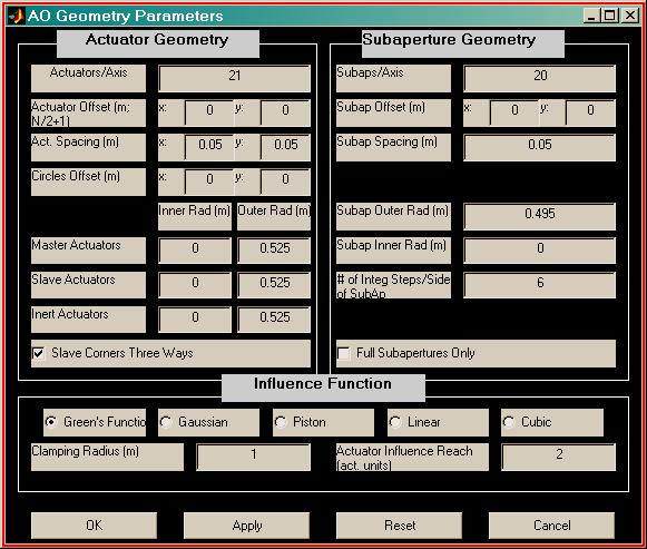
It is in this window that most of the activity of aogeom occurs. The user edits the various entries to modify the characteristics of the AO system geometry. While working with these items, the main window diagram is not automatically updated. Instead the user must press the , , or buttons. The button causes all changes to window to be committed and closes the window. commits the changes but leaves the window open and reloads the default configuration and leaves the window open. closes the window while discarding the changes that were made since the last apply.

In the AO Geometry Parameters window, the user specifies meshes of actuators and subapertures by specifying
(1) actuator and subaperture mesh offsets and dimensions;
(2) the radii of a series of concentric circles that restrict the meshes to specified annuli.
The user usually creates a configuration which consists of an array of subapertures whose corners coincide with an array of master actuators (the Fried geometry). The master actuators are intended to be directly driven by the inversion of a wavefront measurement over the subapertures. The user can also set up inner and outer rings of "slave" actuators. The slave commands are constructed as fixed linear combinations of neighboring master actuators, rather than from the slope pseudo-inversion procedure directly. Finally, aogeom also has a provision for rings of "inert" actuators (BUT see the WARNING below).
The following two figures illustrate the setup of an AO system geometry which includes master, slave, and inert actuators superposed on an annular aperture. For graphical completeness, a non-zero number of inert actuators have been included in this picture, despite the WARNING below. This new system geometry was obtained by editing the default geometry of the previous Geometry Parameters window.

The two red circles show the inner and outer boundaries of the subapertures. In the above example, any subaperture that falls mostly between the inner and outer subaperture radii is included. The "Full Subapertures Only" option (AO Geometry Parameters window, Subaperture Geometry box) will result in inclusion of only those subapertures that fall completely between the inner and outer subaperture radii.
The two white circles show the inner and outer boundaries of the master actuators.
The two magenta circles show the inner and outer boundaries of the slave actuators.
The two green circles show the inner and outer boundaries of inert actuators.
The outermost, cyan circle shows the clamping radius for the Green's function method (if that influence function is selected).

WARNING regarding inert actuators: the purpose of defining "inert" actuators was to model an unfortunate but potentially important event that occurs with physical DMs. Component failures can cause individual actuators to become inactive, in the sense that applying a voltage to that actuator produces no displacement. Since a DM is generally a high-value component, a working optical system that contains a DM with some dead actuators will usually continue to be used as is, at least for some time. Therefore, simulating the performance impact of dead actuators may be an important task. However, at present, the AO tools lack a consistent treatment of this issue in two respects. First, since dead actuators can occur anywhere in any grouping, the "ring" geometry currently provided by aogeom is inappropriate. Second, the present reconstructor calculations do not correctly handle the behavior of the dead actuators. We intend to add the required extensions to the AO tools, but, for the time being, users should only create DM configurations with zero inert actuators. (This is done by making the circle radii for inerts and slaves equal, i.e., specifying zero-width inert rings).

Note that the View menu in the aogeom window must be used to turn on/off display options such as the text labels and boundary circles. The colored legend at the upper right of the geometry picture indicates the total count of each type of actuator and the number of subapertures. The rings of actuators and subapertures shown in the previous picture were generated by specifying the eight radii contained in the Geometry Parameters window located immediately below.

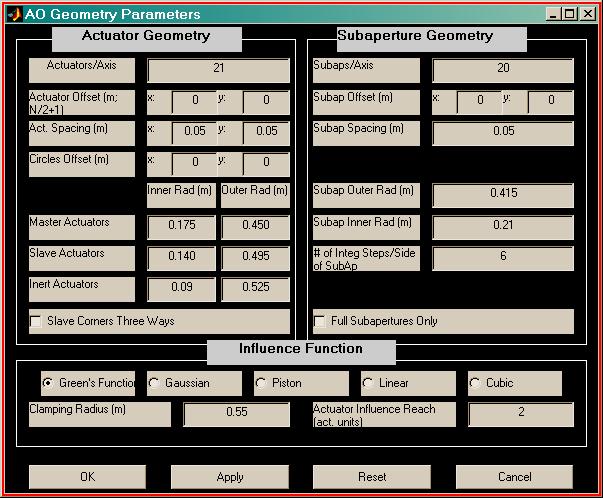
The number of actuators and subapertures per axis define an initial rectangular array which is circumscribed by the circles. The precise values of circle radii are only important insofar as they exclude or include particular actuators or subapertures. As a matter of convention, we usually place an actuator at the origin, and we make the number of actuators along an axis odd so that the system is symmetric. The number of subapertures per axis is usually even and one less than the number of actuators. These conventions are not limitations of the underlying mechanisms; they simply set out a standard way of setting up the systems. The x-dimension is the horizontal axis in the aogeom diagram, and the y-dimension is the vertical axis.

Also specified are the actuator and subaperture spacing. These values indicate the distance between actuators and the distance between centers of subapertures. Actuators can be spaced differently in x and y, but subapertures cannot (note there are no separate x and y subap spacing specs in the above diagram). Usually the x and y spacing of actuators and subapertures are equal (as illustrated). See the background section for further comments on asymmetry and misregistration. The actuators, subapertures, and circle centers are normally symmetric with respect to the origin of the coordinate system. However, the user can specify offsets to any of these. For the definitions of each offset, see the subsequent section on aogeom details.

The yellow lines connecting the magenta and white diamonds illustrate the slaving relationship between master and slave actuators. The yellow lines drawn from the slaves to the masters show upon which masters the slave actuators depend. In the illustrated case, a master-slave connection algorithm which connects slaves to only one or two masters is used. The Slave Corners Three Ways option can be used to cause slaves to be connected to up to three adjacent masters.

Actuator and subaperture numbering convention

If the user wishes to work with some of the intermediate variables in the AO configuration process, it will be necessary to understand the 1-dimensional numbering convention for actuators and subapertures that is used by the AO tools. For actuators, the convention is that actuator 1 is at the left end of the bottom row of actuators (as seen in aogeom diagram). The actuator number increases going from left to right across the rows, and then up the rows from bottom to top. By using the menu option View - Show Actuator Numbers in the aogeom window, the numbers can be displayed.

The numbering of subapertures follows a different pattern than the actuators. For subapertures, the convention is that subaperture 1 is at the bottom of the left-most column. Then subaperture number increases going from bottom to top along the columns, and then across the columns from left to right.

Awareness of the numbering scheme is not required for working with the aogeom GUI, but the data vectors saved to file by aogeom are ordered according to these conventions. For example, there are vectors that contain the x and y coordinates of actuators and subapertures. To work with some of the intermediate variables in the AO tools, the user should be aware of the numbering conventions.

Specifying the actuator influence function and its parameters

Finally, the characteristics of the actuator influence function are also specified in the AO Geometry Parameters window. These specifications do not affect the display of the geometry, so there is no graphical feedback. The user simply selects one of five different influence functions, and specifies the extent of the influence function in a manner unique to each influence function type. The option details are described later.

Saving the results of aogeom

When users are satisfied with the specified AO system geometry, they can store the configuration to a .mat file, using the FileSave As... command in the file menu of the main aogeom window. The file can be loaded into a later run of aogeom (using FileLoad ...) for further editing, and/or provided as input to aoinf and/or other AO tools procedures. The save file name is entirely user-specifiable. Contents of the save file are detailed in .mat Interface File Contents.

aogeom - Details

This section reviews each entry field in the AO Geometry Parameters dialog window, and specifies some details not discussed previously. As seen in the previous examples, the dialog window is separated into three parameter specification sections (Actuator Geometry, Subaperture Geometry, and Influence Function) plus a control buttons section at the bottom of the window. The entries in the parameter specification sections determine the geometry of the system, the relationship of slave to master actuators, and the type of influence function.

Actuator geometry entries

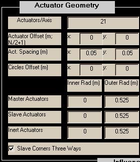
Actuators/Axis: The actuators are assumed to be distributed on a rectangular (usually square) mesh clipped by an annular region. Actuators/Axis is usually set to the number of actuators across the widest part of the aperture. This figure should include all actuators master, slave, and inert. A conventional choice would be to place an actuator at the origin, with two lines of actuators lying on the x and y axes and the remaining actuators distributed symmetrically about the x and y axes: to do this, begin with Actuators/Axis = odd integer.

Actuator Offset: Specifies the (x,y) offset, in meters, of the center of the actuator mesh from the local (x,y) origin. If Actuators/Axis is odd, the "center of the actuator mesh" corresponds to the center actuator. If Actuators/Axis is even, the "center of the actuator mesh" is halfway between the two middle actuators.

CAUTION: regarding alignment between actuators and subapertures, see the background section for comments on asymmetry and misregistration.

Act. Spacing: Specifies the x and y spacing, in meters, between actuators. The x and y spacings are usually, but not necessarily, made equal. As discussed previously, this specification is usually made in object space coordinates.

Circles Offset: The radii specified below define circles nominally centered at the local origin. "Circles offset" provide a means to shift the centers of these circles relative to the local origin. All offsets and radii are specified in meters.

Various Actuator Radii: In specifying the actuator geometry, the user sets up annular regions used to indicate boundaries for different types of actuators. These regions are superposed on the mesh of actuators and used to clip or type each actuator. For each type of actuator there are two radii. Let r_master and R_master be the inner and outer radii of the master actuators, respectively. Similarly let r_slave, R_slave, r_inert, and R_inert be the inner and outer radii of the slave and inert actuators. The system must be set up such that

R_inert >= R_slave >= R_master > r_master >= r_slave >= r_inert >= 0.

Given the array of actuators and the offsets defined above, all actuators falling outside the circle of radius R_inert or inside the circle of radius r_inert are eliminated from the configuration. Actuators falling between R_inert and R_slave and r_inert and r_slave are deemed inert actuators. Actuators falling between R_slave and R_master and r_slave and r_master are deemed slave actuators. Finally, actuators falling between R_master and r_master are identified as master actuators.

Note in particular that if R_inert=R_slave , then there will be 0 inert actuators at the outside edge of the mirror. Likewise, if r_slave=r_inert, then there will be 0 inert actuators in the inner annulus.

Slave Corners Three Ways: aogeom provides two ways of automatically setting up master-slave relationships depending on slave and master adjacencies. When the 3-ways box is not checked, slaves which are on a corner adjacent to three actuators, one vertically, one horizontally, and one diagonally, are only slaved to the horizontal and vertical actuators. If the slave is on a side which is vertically or horizontally adjacent to one master and diagonally adjacent to two actuators, the actuator is slaved only to the vertical or horizontal master. In the annular region, the slaving occurs in such a way that horizontal and vertical slaves are favored and diagonal slaves are not used if a horizontal and/or vertical masters are available. When the 3-ways box is checked, slave actuators are slaved to every adjacent master actuator, vertical, horizontal, and diagonal.

Subaperture geometry entries

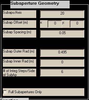
Subaps./Axis: The subapertures are assumed to be distributed on a square mesh clipped by an annular region. Subaps/Axis is usually set to the number of subapertures across the widest part of the aperture. A conventional choice would be to begin with Subaps/Axis equal to one less than Actuators/Axis.

Subap. Offset: Specifies the (x,y) offset, in meters, of the center of the subaperture mesh from the local (x,y) origin. If Subaps/Axis is even, the "center of the subaperture mesh" is a corner where four subapertures meet. If Subaps/Axis is odd, the "center of the subaperture mesh" is the center of the middle subaperture.

CAUTION: regarding alignment between actuators and subapertures, see the background section for comments on asymmetry and misregistration.

Subap. Spacing: Specifies the x and y spacing, in meters, between subaperture centers. Only equal x and y spacing is allowed for the subapertures. Furthermore, the width of the subapertures is assumed equal to the spacing (i.e., 100% fill factor). To deviate from the 100%-fill square subapertures, see the comments in the background section. As discussed previously, this specification is usually made in object space coordinates.

Subap. Radii: In specifying the subaperture geometry, the user sets up annular regions used to indicate boundaries for the subapertures. These regions are superposed on the mesh of subapertures and used to clip the subapertures. Let r_subap and R_subap be the inner and outer radii of the master actuators, respectively. Subapertures which fall outside R_subap or inside r_subap are eliminated. Usually r_subap and R_subap are approximately equal to R_master and R_master because it is natural to set up the AO system so that master actuators are at the every corner of every subaperture. In fact, reconstructors computed for systems which contain a master actuator not located at the corner of a sufficiently-illuminated subaperture or a slave actuator at the corner of a sufficiently-illuminated subaperture will be poorly conditioned.

# of Integ. Steps/Side of Subap.: When computing the slope influence function, aoinf numerically evaluates the G-tilt formula over a subaperture area. The integration rule that is used requires the parameter "# of Integ. Steps/Side of Subap." to be EVEN. Six or eight should be sufficient to represent the shape of a deformed mirror over the region of a subaperture.

Full Subapertures Only: This selection determines the method of excluding and including subapertures within the specified subaperture radii. When this option is not selected, any subaperture whose area lies mostly between the inner and outer subaperture radii will be included. When this option is selected, only subapertures whose area falls completely between the radii are included.

Influence function entries

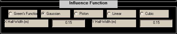
In this section of the Parameters window, the user specifies the shape and extent of the single-actuator influence function. The user has the choice of five shapes: Green's Function, Gaussian, Piston, Linear, and Cubic. For each shape the user is prompted for two parameters that define the effective width of the influence function. This section describes each influence function shape and the corresponding width parameters. To choose a particular influence function shape, the user chooses the appropriate button, and then enters the width information in the resulting editable text boxes. Since the Green's function influence shape is directly based on a physics equation that describes the mechanical properties of a flexible plate, it is probably a more accurate representation than the empirical options (gaussian, piston, linear, cubic). However, if the width parameter is not well known, then the superiority of the Green's function shape over some of the empirical ones is questionable.

Except for the Green's Function clamping radius, the specification of the influence function has no impact on the graphical representation of the AO system geometry. It simply sets up input parameters which are used by aoinf in its calculation of the influence function matrices. So, as far as calculations are concerned, the following description of the influence functions is more relevant to aoinf rather than aogeom. Nevertheless, we classify the specifications as geometry information, and therefore the specs are entered in the aogeom GUI.

Green's Function:

The so-called "Green's function" influence function in aoinf is derived from the solution of a clamped-plate partial differential equation (Balakrishnan). The user specifies two input parameters:
(1) the clamping radius, r_clamp, in m
(2) the number of actuators away that a given actuator affects ("actuator influence reach"), in actuator units.
Beyond this reach, the influence function is assumed to be identically zero: this is a practical concession to limit the size of the influence function matrix. Since the Green's function influence shape is directly based on a physics equation that describes the mechanical properties of a flexible plate, it is probably a more accurate representation than the empirical options (gaussian, piston, linear, cubic) described below. To date, the Green's Function shape has been the choice most commonly used by MZA modelers when applying WaveTrain.

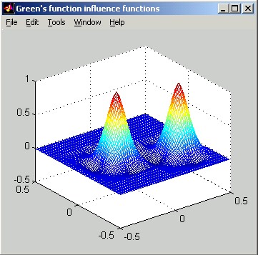
The following slice plot shows Green's influence functions far from the clamping radius and near the clamping radius. The spacing between actuators is 0.15 m, and the actuator influence reach is 2 actuators. The horizontal distance scale of the slice plot is in meters. The vertical scale can be interpreted as relative: the poked actuator has been displaced by 1 unit.

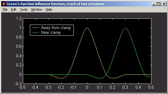
Notice that the negative deflection of the surface on the right side of the actuator near the clamp is different than the deflection far from the clamp. Although clamped DMs appear to be a thing of the past, this formulation can still be used for modern DMs by specifying r_clamp >> r_inert , to model an essentially unclamped DM. Qualitatively, the Green's function solution differs from all the other influence function options in that it produces negative deflection lobes at certain distances from the force application point.

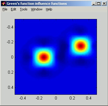
The two pictures below show image-plot and perspective-plot representations equivalent to the above slice plot.

REFERENCES:

A.V. Balakrishnan, "Shape control of plates with piezo actuators and collocated position/rate sensors", Applied Mathematics and Computation, vol. 63, pp. 213-234, 1994.

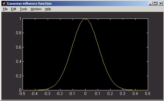
Gaussian:

Gaussian influence functions implement the form:

d = exp(-Dx²/w_x²) * exp(-Dy²/w_y²)

where

w_x    is the X Half Width at the 1/e point, specified by the user in aogeom,
w_y    is the Y Half Width at the 1/e point, specified by the user in aogeom,
Dx    is the distance in x from the poked actuator, at the point where the surface deflection is to be determined,
Dy    is the distance in y from the poked actuator, at the point where the surface deflection is to be determined,
d   is the surface deflection at the point located (Dx,Dy) from the poked actuator.

Usually, w= w_x= w_y , which, for Dr² = Dx² + Dy² means:

d = exp(-Dr²/w²).

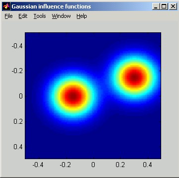
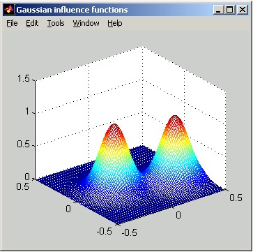
The following figures illustrate Gaussian influence functions. The horizontal distance scale of the slice plot is in meters. The vertical scale can be interpreted as relative: the poked actuator has been displaced by 1 unit.

Piston:

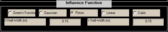
Piston influence functions implement the form:

d = 1 when |Dx| < w_x and |Dy| < w_y, and 0 otherwise

where

w_x    is the X half-width specified by the user in aogeom,
w_y    is the Y half-width specified by the user in aogeom,
Dx    is the distance in x from the poked actuator, at the point where the surface deflection is to be determined,
D y    is the distance in y from the poked actuator, at the point where the surface deflection is to be determined,
d     is the surface deflection at the point located (Dx,Dy) from the poked actuator.

The following figures illustrate Piston influence functions. The horizontal distance scale of the slice plot is in meters. The vertical scale can be interpreted as relative: the poked actuator has been displaced by 1 unit.

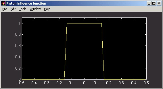
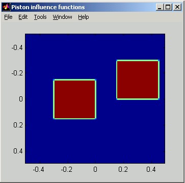
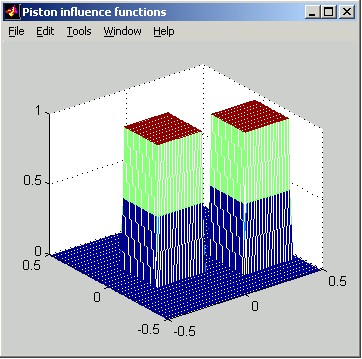
Linear:

Linear influence functions implement the form:

d = (1 - |Dx|/w_x) * (1 - |Dy|/w_y), when |Dx| < w_x and |Dy| < w_y, and 0 otherwise,

where

w_x    is the X half-width (to the zero point) specified by the user in aogeom,
w_y    is the Y half-width (to the zero point) specified by the user in aogeom,
Dx    is the distance in x from the poked actuator, at the point where the surface deflection is to be determined,
D y    is the distance in y from the poked actuator, at the point where the surface deflection is to be determined,
d   is the surface deflection at the point located (Dx,Dy) from the poked actuator.

The following figures illustrate Linear influence functions. The horizontal distance scale of the slice plot is in meters. The vertical scale can be interpreted as relative: the poked actuator has been displaced by 1 unit.

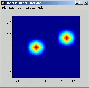
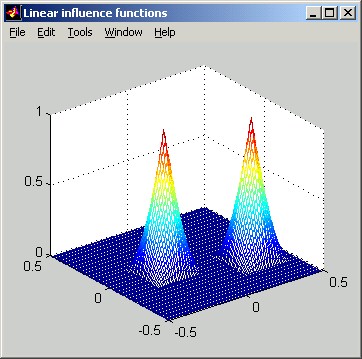
Cubic:

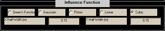
Cubic influence functions implement the form:

d_x = (1-(Dx/w_x)²)(1-(Dx/(2w_x)))   when Dx < w_x,
     = ((Dx/w_x)² - (Dx/w_x))(2 - (Dx/w_x))   when w_x < Dx < 2w_x,
     = 0   when Dx > 2w_x,
d_y = (1-(Dy/w_y)²)(1-(Dy/(2w_y)))   when Dy < w_y,
     = ((Dy/w_y)² - (Dy/w_y))(2 - (Dy/w_y))   when w_y < Dy < 2w_y,
     = 0   when Dy > 2w_y ,
d = d_x d_y.

where

w_x    is the X half-width specified by the user in aogeom,
w_y    is the Y half-width specified by the user in aogeom,
Dx    is the distance in x from the poked actuator, at the point where the surface deflection is to be determined,
D y    is the distance in y from the poked actuator, at the point where the surface deflection is to be determined,
d   is the surface deflection at the point located (Dx,Dy) from the poked actuator.

The following figures illustrate Cubic influence functions. The horizontal distance scale of the slice plot is in meters. The vertical scale can be interpreted as relative: the poked actuator has been displaced by 1 unit.

Review of Control Buttons:

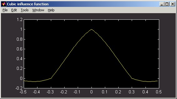
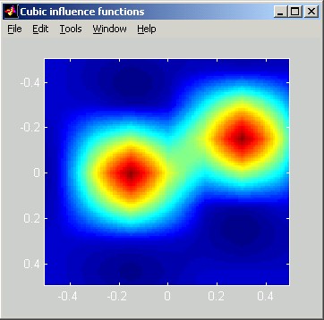
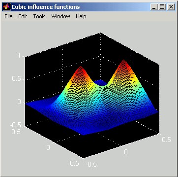
While working in the AO Geometry Parameters window the main window diagram is not automatically updated. Instead the user must press the , , or buttons. The button causes all changes to window to be committed and closes the window. commits the changes but leaves the window open and reloads the default configuration and leaves the window open. closes the window while discarding the changes that were made since the last Apply.

Pictorial elements of the AO geometry diagram

This section summarizes the elements of the AO system geometry graphical display.

Axes: Indicate the coordinates and sizes of actuators, subapertures, and annular regions.

Red Circles: Subaperture inner and outer radii.

White Circles: Master actuator inner and outer radii.

Magenta Circles: Slave actuator inner and outer radii.

Green Circles: Inert actuator inner and outer radii.

Cyan Circle: The Green's function clamping radius when Green's function influence function is used. The clamping radius is often so large that it is outside the range of the displayed axes.

Red Squares: Subaperture regions.

White Diamonds: Master actuators.

Magenta Diamonds: Slave actuators.

Green Diamonds: Inert actuators.

Yellow Lines: Dependencies of slave actuators on particular master actuators.

Legend: Number of inert, slave, and master actuators, followed by the number of subapertures.

Matlab Function Details: Computing Influence Function and Reconstructor Matrices

This section gives syntax details and usage examples for all the AO tools functions that have been identified in the background discussion pertaining to influence and reconstructor matrices.

aoinf

Using data generated by aogeom (or a user-supplied equivalent), aoinf computes the DM's OPD and slope influence function matrices. aoinf is a utility that can be accessed either from Matlab or from the operating system console window. Most users will access aoinf from Matlab.
aoinf generates a .mat file that saves the results of aoinf 's calculations; the same output file also resaves all the geometry data read in from the aogeom output file.

From the operating system console window the calling syntax for aoinf is:

C> aoinf infilespec outfilespec nxopd dxopd

From Matlab the calling syntax is:

>> aoinf(infilespec, outfilespec, nxopd, dxopd);

where

infilespec = name of .mat input file from which the AO geometry specifications are to be read. Usually, but not necessarily, this file is created by aogeom. The filename specification must include the .mat suffix.

outfilespec = name of .mat file to which the resulting combined influence functions and AO geometry are to be written. This file can later be loaded into Matlab for computation of the reconstructor using aorecon, or specified as a constructor argument to TasatDMModel. The filename specification must include the .mat suffix.

nxopd = number of points across the square mesh superimposed on the DM for the purpose of resolving surface deflections on the OPD mesh. This number, together with dxopd, must span the entire mirror (but not the entire propagation mesh). The OPD mesh is a "gwoom" type (see the WaveTrain User Guide discussion of coordinate systems and meshes). The origin lies at the nxopd/2 + 1 point (counting from 1). Hence, the mesh is not quite symmetric, and one must be careful to use nxopd and dxopd combinations which covers the entire physical region of interest.

dxopd = physical spacing (in m) between mesh points of the square mesh superimposed on the DM for the purpose of resolving surface deflections on the OPD mesh. This parameter needs to be small enough to properly model the shape of the mirror and ought to be smaller than the spacing between actuators. It is usually sufficient to use six to twelve points per actuator spacing. CAUTION: the actuator spacing MUST BE an integer multiple of dxopd (it is suggested that dxopd be input in the format [dxact]/N ).

Notice that aoinf has no output arguments: all outputs are saved to outfilespec.
Key results computed by aoinf are saved under the following names:
opdif = DM OPD influence function matrix: maps actuator displacements in meters
             to DM surface displacements in meters. The surface displacements may be
             defined on a substantially denser mesh than the actuators.
dtos and mvtos = two closely-related slope influence function matrices, where:
     dtos = slope influence matrix that maps all actuator displacements to all slopes
                 (mapping meters to tilt angle in radians of angle).
     mvtos = slope influence matrix that maps master actuator volts to all slopes.
                    Usually we treat volts as equal to displacements, so that mvtos maps
                    meters to tilt angle in radians of angle.
                    For a review of the use of masters and slaves, and volts and displacements,
                    see the background section on influence functions. An important point to bear
                    in mind is that mvtos is the matrix that should be pseudo-inverted by aorecon.

By loading outfilespec into the Matlab workspace, the user can inspect and work with the above-mentioned influence matrices. The names and formats of all the saved variables are summarized in the section .mat Interface File Contents. Remember that, in addition to the influence matrices, outfilespec will also contain all the preceding data saved by aogeom. This redundancy is convenient, and uses little extra storage, since the aogeom data is small compared to the influence matrices.

CAUTION: Two execution errors that users may encounter with aoinf are due to:
(a) the specified dxopd does not divide the actuator spacing an integral number of times;
(b) the nxopd, dxopd combination does not entirely cover the mesh of actuators.
Recommended ways of avoiding these error conditions are:
(a) Specify dxopd as an integer divisor of the actuator spacing (i.e., dxopd = dxact/N, where dxact is the actuator spacing and N is an integer)
(b) Carry out a preliminary setup check, using the Matlab utility function opdc to generate OPD coordinates, and construct a composite plot with the xact, yact, xsub, and ysub coordinates that are supplied by the aogeom output file.
Starting with a sample file generated by aogeom, the following Matlab example illustrates the use of the recommended setup check procedure:

>> load small45g    % Load a .mat file previously created with aogeom.
>> dxact=max([xact(2)-xact(1),yact(2)-yact(1)]);    % This determines the actuator spacing.
>> dxopd=dxact/5;    % dxopd is an integral divisor of dxact.
>> nxopd=32;
>> xopd=opdc(nxopd,dxopd); % Generate a coordinate vector.
>> [x,y]=meshgrid(xopd,xopd);    % Generate a coordinate mesh.
>> plot(x(:),y(:),'.')    % Plot the mesh with blue dots.
>> axis square    % Make the plot area square.
>> hold on;plot(xact(:),yact(:),'r+')    % Plot the actuators with red plusses.
>> hold on;plot(xsub(:),ysub(:),'ks')    % Plot the subaperture centers with black squares.
>> hold off;

In this case the following plot is generated:

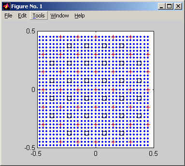
What we are looking for is to ensure the actuators (+) lie on the OPD mesh points (blue dots). Also we want to make sure that the blue dots cover the entire region covered by the actuators. The locations of the center of the subapertures, but not the sizes, are indicated by the black squares. From this plot we expect that nxopd and dxopd ought to be valid inputs to aoinf.

The following sequence illustrates a successful execution of aoinf, using the above input parameters:

>> dxact=max([xact(2)-xact(1),yact(2)-yact(1)]);    % This determines the actuator spacing.
>> dxopd=dxact/5;    % dxopd is an integral divisor of dxact.
>> nxopd=32;
>> aoinf('small45g.mat','small45gi.mat',nxopd,dxopd) % Run aoinf
Warning: the variable balmodel was not found in file small45g.mat
     (% This warning message should be ignored).
aoinf: Reading DM specification from: [small45g.mat].
aoinf: Writing DM matrices to: [small45gi.mat].
aoinf: Using a mesh with 32 points and 0.030000 spacing.
aoinf: Completed successfully.

The following sequence illustrates an unsuccessful execution of aoinf, due to poor specification of nxopd (not enough points to cover the entire mesh of actuators):

>> dxact=max([xact(2)-xact(1),yact(2)-yact(1)]); % This determines the actuator spacing.
>> dxopd=dxact/5; % dxopd is an integral divisor of dxact.
>> nxopd=30; % This is not large enough to cover all the actuators.
>> aoinf('small45g.mat','small45gibad.mat',nxopd,dxopd)
Warning: the variable balmodel was not found in file small45g.mat
aoinf: Reading DM specification from: [small45g.mat].
aoinf: Writing DM matrices to: [small45gibad.mat].
aoinf: Using a mesh with 30 points and 0.030000 spacing.
aoinf: Error reading or generating DM.
aoinf: Aborted with error number -896.

CAUTION: aoinf can bog down when the user has specified a problem that requires too much CPU and/or memory. In this case, aoinf takes what seems to be forever to complete. The aoinf computation can be rather time-consuming, but should probably not take more than fifteen minutes or so. If the processing does continue longer, the user should probably rethink the actuator influence reach and/or the OPD mesh spacing. The OPD influence function is nominally dimensioned nact x nxopd², which can of course be very large. (Note that nxopd² = n_opd as defined in the background section on OPD influence functions.) To ameliorate the size problem, aoinf stores the influence function in a sparse form, which takes advantage of the fact that any given actuator affects only a small subset of the OPD points (the vast majority of matrix elements are 0). This allows reasonable sized OPD influence function matrices to be created. If the number of OPD points affected by a given actuator is large, the computation will take a long time and the resulting file will be large.

lsfptos

Using data generated by aogeom (or a user-supplied equivalent), lsfptos computes a slope influence function matrix which can be used for wavefront sensing in the absence of a DM. In this case the aoinf routine is not used. We still set up the WFS geometry with aogeom, but then we continue with the sequence lsfptos-aorecon, instead of using the sequence aogeom-aoinf-aorecon. When we use lsfptos in the absence of a DM, "actuator" locations specified in aogeom are interpreted as the points at which the wavefront OPD is represented. lsfptos requires that the "actuator" locations be at the corners of the subapertures.

From the Matlab command line, the calling syntax for lsfptos is:

>> [ptos, c] = lsfptos(xsub, ysub, xact, yact); % NOTE: the first letter of "lsfptos" is lower case "ell"

where

xsub   = vector (dim n_sub x 1) containing the x-coordinates (in m) of the centers of the WFS subapertures. The subaperture numbering convention has been described previously.
ysub   = vector (dim n_subx 1) containing the y-coordinates (in m) of the centers of the WFS subapertures.
xact   = vector (dim n_actx 1) containing the x-coordinates (in m) of the "actuator" locations. The actuator numbering convention has been described previously.
yact   = vector (dim n_actx 1) containing the y-coordinates (in m) of the "actuator" locations.

ptos = the slope influence matrix of type S'_c, defined previously. Dimensions are 2n_sub x n_act .

CAUTION: the lsfptos routine neglects to divide by the actuator separations dx_act and dy_act when computing the matrix ptos. To compensate manually, see the Matlab example listed next.
UNITS: after the compensating divisor is applied, the corrected matrix ptos will map an OPD vector in units of meters into a slopes vector in units of radians of tilt angle.

c = diagnostic quantity not needed for subsequent processing.

Starting with a sample file generated by aogeom, the following Matlab example illustrates the use of lsfptos:

% First, use aogeom to inspect the subap and "actuator" layout to be used:
>> aogeom
        % Using File-Load in the AOgeom window, load "small45g.mat" into the geometry display
        % Note that we have 32 subapertures and 45 "actuators" in this configuration.
        % Using File-Define Geometry, inspect the Parameters window: note that the "actuator"
        % spacing dx_act = 0.15m = dy_act.
% Now load "small45g.mat" into the Matlab workspace:
>> load small45g.mat
         % The coordinate vectors xact, yact, xsub, ysub are now present in the workspace;
         % xact and yact have dim (45x1), xsub and ysub have dim (32x1).
>> [ptos,c] = lsfptos(xsub, ysub, xact, yact);   % Compute the S'_c matrix, absent a scale factor.
>> ptos = ptos/0.15;   % Divide by the actuator spacing (in m) to correct for the missing scale factor.

% For testing purposes, we now create an opd map at the "actuator" coordinates.
% The functional form of the opd will be a uniform tilt, with x-tilt = 1E-6 rad, and y-tilt = 2E-6 rad,
% expressed by the equation opd = (x / 1.0m)*1E-6m + (y / 1.0m)*2E-6m, where {x,y,opd} are in m:
>> for k=1:nact; opd(k,1) = ( xact(k)/1.0)*1E-6 + (yact(k)/1.0)*2E-6; end;
% Note that opd must be defined as a column vector, dim (n_actx1) =( 45x1).

% Now apply the slope influence matrix S'_cto compute subaperture slopes:
>> s = ptos*opd;
         % s is the vector of subaperture slopes (dim 2n_sub x 1 = 64x1) in radians of angle,
         % where s(1:32) are the x-slopes, s(33:64) are the y-slopes.
>> s(1:32)';     % Print the x-tilts in each subap: each is 1E-6 rad, as expected.
>> s(33:64)';   % Print the y-tilts in each subap: each is 2E-6 rad, as expected.

aorecon

The function aorecon computes the pseudo-inverse of a specified matrix, with a variety of options. The matrix to be pseudo-inverted may be generated by aoinf, lsfptos, or some user-supplied analogue. aorecon can compute either tilt-included or tilt-removed reconstructors, and can perform singular value decomposition to suppress near-singular modes. One uses aorecon to carry out different tasks by calling the routine several times, each time with a different argument syntax.

Since aorecon is often the last step in the AO configuration process (see the summary table), it will be convenient to create a save file that contains any reconstructor matrices generated by aorecon plus all the previous variables created by whatever combination of aogeom, lsfptos, aoinf, and other routines was used. Since some of the variables of interest have been saved previously in other files, this creates some redundancy. However, for purposes of later rework or for insertion into a WaveTrain simulation run, we recommend to collect all relevant variables into one final .mat save file. Because of the number of options available, there is no convenient way for the aorecon function to do this for the user: the user must manually create the save file using Matlab's easy-to-use "save" command. An example is given in one of the following Matlab session examples. To reduce keyboard tedium, the recommended procedure is to save the whole workspace (perhaps after deleting certain temporary work variables that the user has no wish to save).

From the Matlab command line, the possible calling syntaxes for aorecon are:

>> rsv = aorecon(M); % Compute singular values of input matrix

where
M = matrix whose singular values are to be computed
rsv = vector of singular values

>> recon = aorecon(M, ns, tiltopt); % Compute "pseudo-inverse" matrix of M

where
M = matrix whose pseudo-inverse is to be computed
ns = number of singular modes to be removed (may be 0)
tiltopt = 0: compute tilt-included pseudo-inverse
1 or OMITTED: compute tilt-removed pseudo-inverse
recon = pseudo-inverse of input M, subject to ns and tiltopt

UNITS associated with recon are dictated by the input matrix M. That is, if M maps OPD in meters to slope angles in radians of angle, then its pseudo-inverse maps slope angle in radians to OPD in meters.

In the following subsections, we illustrate two applications of aorecon, and we exercise several of the options.

Application to zonal reconstruction of wavefront (no DM)

Here we show how aorecon is used to operate on the output of lsfptos. This produces a zonal reconstruction of a wavefront from slope data, in the absence of a DM. The following sequence of Matlab commands illustrates the procedure. For the origin of the Matlab variables used below, refer to the Matlab excerpt in the section on lsfptos.

% First, we pseudo-invert (including SVD) the S'_c slope influence matrix that was computed by lsfptos :
>> rsv = aorecon(ptos);   % Calculate the vector of singular values rsv.
The reconstructor WAS NOT computed by this function call.
>> figure; semilogy(rsv,'o-');   % Inspect rsv to determine how many singular values should be suppressed:
                                         % see the graph and discussion below.
>> ns = 2;   % From inspection of the plot, it appears we should remove two singular modes.
>> reconti = aorecon(ptos,ns,0);   % Compute the tilt-included reconstructor, dim (45x64).

Singular value decomposition: Choosing the number of singular values to remove may not be entirely obvious. The vector rsv usually contains steadily decreasing values which span several orders of magnitude. When there are near-singular modes, there is usually an obvious break point at which the values suddenly drop by several orders of magnitude. The typical result for AO systems appears to be a few near-singular modes which occur towards the end of the vector. In the following plot, we show the singular values of the above ptos matrix. As noted in the Matlab command comments, the plot behavior suggests we should remove two modes:

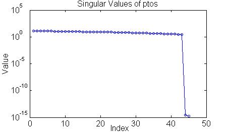
% We now continue the Matlab example, assuming that the s vector generated in the lsfptos example represents empirical WFS slope data, in radians of angle, from which we will reconstruct the wavefront opd in units of m:
>> opdrec = reconti*s;   % Compute vector of reconstructed OPD values, at the "actuator" locations.
                                       % opdrec has dim (n_actx1)=(45x1), and units of m.
>> figure; plot(opdrec - opd);    % To check the solution, plot the difference between the reconstructed WF and the truth WF, vs. "actuator" index. The plot (not shown here) shows that the difference is tiny, which indicates an accurate reconstruction.

% When working with real WFS data, we often want to make a mesh or image plot of the reconstructed wavefront. The utility function actmap can be used to prepare the OPD vector for this purpose:
>> opdrec2d = actmap(opdrec, xact, yact); % Output opdrec2d is the (nx_actx ny_act) array that
% rearranges vector opdrec into its 2D layout.
>> figure; imagesc(opdrec2d); axis image; colorbar; xlabel('Y index'); ylabel('X index');
% The resulting image plot is reproduced below. It verifies that the reconstructed WF is a tilted plane with 1 urad of x-tilt, and 2 urad of y-tilt, in agreement with the original WF from which the slope data was constructed (see lsfptos example). In the corners, where there were no "actuators", a default value of OPD equal to the bottom of the color scale was assigned.

Application to zonal reconstruction of DM actuator commands

Here we show how aorecon is used to operate on the output of aoinf. This produces a zonal reconstruction of DM actuator commands from slope data. The following sequence of Matlab commands illustrates the procedure.

>> load small45gi.mat;   % Load the output file of aoinf into a clean Matlab workspace.
                                         % (The user need not generate this file: it is provided as an
                                         % example file in the WaveTrain distribution.)
>> rsv = aorecon(mvtos);   % Calculate the vector of singular values rsv.
The reconstructor WAS NOT computed by this function call.
>> figure; semilogy(rsv,'o-');   % Inspect rsv to determine how many singular values should be suppressed:
                                         % see the graph and discussion below.
>> ns=1;   % From inspection of the plot, it appears we should remove one singular mode.
>> recon   = aorecon(mvtos,ns);      % Compute the tilt-removed reconstructor.
>> reconti = aorecon(mvtos,ns,0);   % Compute the tilt-included reconstructor.
>> save small45gir.mat    % Save the resulting workspace as a *.mat file named "small45gir.mat".
                                          % The file name can be arbitrarily specified by the user.
                                          % NOTE regarding the save file: in contrast to running aoinf, running aorecon does not automatically create a save file. This behavior was chosen because of the number of options that aorecon has. Saving the entire workspace in the above example results in the creation of a single data file with all the data that could be needed by a WaveTrain simulation run. Of course if the user has created extra working variables in the Matlab session, these may be deleted if desired before saving. However, the presence of extra variables in the save file does no harm. This final save file, which will contain the previously-loaded AO geometry data, the influence function matrices, and one or more reconstructor matrices can be rather large (easily several 10s of MB).

Note that the slope influence-function input to aorecon is the matrix mvtos. As explained in a background section, "volts" are by default equivalent to "displacements" because the current default mapping of actuators volts to displacements (matrix vtod) is the unit matrix.

Singular value decomposition: Choosing the number of singular values to remove may not be entirely obvious. The vector rsv usually contains steadily decreasing values which span several orders of magnitude. But when there are near-singular modes, then there is usually an obvious break point at which the values rapidly decrease by one or two orders of magnitude. The typical result for AO systems appears to be a few near-singular modes which occur towards the end of the vector. In the following plot, the singular values of the influence function in small45gi.mat are plotted:

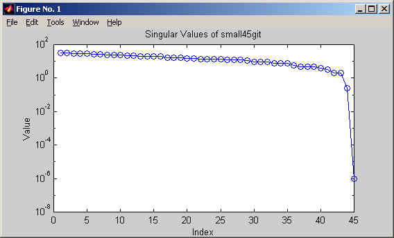
From inspection of the graph, we choose to eliminate 1 singluar mode, because of the drop of more than four orders of magnitude between the 44th and 45th points. One might be tempted to try 2 singular values because of the drop of one order of magnitude between the 43rd and 44th values; but, it has been our experience that one should only suppress the singular values which are roughly of the same order of magnitude as the lowest value.

Variables contained in the output file: As explained at the end of the sample Matlab session, the save file will contain one or more reconstructor matrices, whose names were user-specified, plus all the preceding data created by aogeom and aoinf. The names and format of these variables are defined in the section .mat Interface File Contents.

lsfptosw

lsfptosw is the key element in the computation of a waffle-constrained reconstructor. We can set up the WFS geometry with aogeom, and then we proceed to lsfptosw and aorecon. (As mentioned in the background discussion, explicit attempts to eliminate waffle using lsfptosw may be redundant because of the removal of singular modes using the SVD capability of aorecon: users must experiment with their particular geometries).

From the Matlab command line, the calling syntax for lsfptosw is:

>> [ptosw, c] = lsfptosw(xsub, ysub, 1, xactmas, yactmas); % NOTE: the first letter of "lsfptosw" is lower case "ell"

where

xsub   = vector (dim n_sub x 1) containing the x-coordinates (in m) of the centers of the WFS subapertures. The subaperture numbering convention has been described previously.
ysub   = vector (dim n_subx 1) containing the y-coordinates (in m) of the centers of the WFS subapertures.
1   = specifies a hardwired code option.
xactmas   = vector (dim n_actx 1) containing the x-coordinates (in m) of the master actuator locations. The actuator numbering convention has been described previously.
yactmas   = vector (dim n_actx 1) containing the y-coordinates (in m) of the master actuator locations.

ptosw = slope influence matrix similar to type S'_c, defined previously.

CAUTION: the lsfptosw routine neglects to divide by the actuator separations dx_act and dy_act when computing the matrix ptos. To compensate manually, see the Matlab example listed next.
UNITS: after the compensating divisor is applied, the corrected matrix ptosw will map an OPD vector in units of meters into a slope vector in units of radians of tilt angle.

c = diagnostic quantity not needed for subsequent processing.

Starting with an existing .mat data file included with the AO tools, the following Matlab example illustrates the use of lsfptosw:

% Load a file with an existing geometry and reconstructor:
>> load c:\mza\wavetrain\predata\nop241f.mat
%
% Find the indices of the master actuators:
>> imas=find(actype>0);
%
% Create the slope influence function which includes the
% unsensed waffle terms. Rescale to physical units
>> [ptosw, c] = lsfptosw(xsub, ysub, 1, xact(imas), yact(imas));
» ptosws=ptosw*(2/(ysub(2)-ysub(1)));
%
% Do the SVD and plot:
>> rsv=aorecon(ptosws);
>> figure;
>> semilogy(rsv,'o-')
%
% Remove one singular value. Create the
% tilt-removed and the tilt-included reconstructors:
>> [reconw,rsv]=aorecon(ptosws, 1, 1); %tilt-removed
>> [reconwti,rsv]=aorecon(ptosws, 1, 0); %tilt-included
%
% Create the usual (NO waffle removal) tilt-removed reconstructor;
% it was not included in the original file. Do the SVD:
>> rsv=aorecon(mvtos);
>> figure;
>> semilogy(rsv, 'ro-')
%
% Remove two singular values:
>> [reconti,rsv] = aorecon(mvtos, 2, 0);
%
% Plot and compare to the original reconstructor:
>> figure
>> slopes=[xsub; ysub];
>> plot(recon*slopes);
>> hold on;
>> hold on;plot(reconw(:,1:416)*slopes, 'r');
>> hold on;plot(reconwti(:,1:416)*slopes, 'g');
>> figure
>> slopestilt=ones(416, 1);
>> plot(recon*slopestilt);
>> hold on;plot(reconti(:,1:416)*slopestilt, 'g');
>> hold on;plot(reconw(:,1:416)*slopestilt, 'r');
>> hold on;plot(reconwti(:,1:416)*slopestilt, 'm');
>> hold off;
%
% The following trims the WCR matrices to the right sizes:
>> reconw=reconw(:,1:416);
>> reconwti=reconwti(:,1:416);
%
% Create a combined .mat file that contains the old and the new reconstructors:
>> save nop241temp reconw reconwti reconti
>> clear
>> load nop241f
>> load nop241temp
>> save nop241fwcr

slope2mod

slope2mod implements the modal wavefront reconstructor procedure that uses Gavrielides polynomials.

From the Matlab command line, the calling syntax for slope2mod is:

>> v = slope2mod(orders, xsub, ysub, rad);

where

orders = vector of indices [r1,r2,...,rN ], that specifies the radial order of the Zernike modes to be included in the reconstruction. For any included radial order, all azimuthal (angular) orders are included.
The values r1,r2,...,rN need not be consecutive: any radial order(s) may be omitted. Radial order 1, referring to tilt, is the lowest allowed order.

xsub = vector (dim n_sub x 1) containing the x-coordinates of the centers of the WFS subapertures. The subaperture numbering convention has been described previously.

ysub = vector (dim n_subx 1) containing the y-coordinates of the centers of the WFS subapertures.

rad = radius (in m) of the circle that defines the normalizing radius for the Zernike circle functions. This should match the radius over which the reconstruction is desired.

v = the matrix V that maps measured slopes s_data to Zernike coefficients a_mod, as described previously.
That is, V has the defining property that a_{mod, rec} = V s_data .

mod2opd

mod2opd computes the Zernike function evaluation matrix Z described previously. This matrix works together with the V matrix computed by slope2mod. After slope2mod and mod2opd have been executed, the user can obtain the final reconstructed wavefront by performing the multiplication

d_{opd,
rec} = Z V s_data, where d_{opd, rec} will be in m, if s_data is in rad.

From the Matlab command line, the calling syntax for mod2opd is:

>> z = mod2opd(xopd, yopd, orders, rad, arad);

where

xopd = vector (dim n_opdx 1) containing the x-coordinates of the points at which WF opd estimation is desired. A simple way of generating xopd is to set it equal to the xact vector generated by aogeom, where the "actuator" points have been defined to be at the corners of the subapertures. However, the Zernike expansion may be evaluated at any arbitrary {xopd,yopd} the user cares to specify.

yopd = vector (dim n_opdx 1) containing the y-coordinates of the points at which WF opd estimation is desired. A simple way of generating yopd is to set it equal to the yact vector generated by aogeom, where the "actuator" points have been defined to be at the corners of the subapertures. However, the Zernike expansion may be evaluated at any arbitrary {xopd,yopd} the user cares to specify.

orders = vector of indices [r1,r2,...,rN ], that specifies the radial order of the Zernike modes to be included. For any included radial order, all azimuthal (angular) orders are included.
The values r1,r2,...,rN need not be consecutive: any radial order(s) may be omitted. Radial order 1, referring to tilt, is the lowest allowed order.

rad = radius (in m) of the circle that defines the normalizing radius for the Zernike circle functions. This should match the radius over which the reconstruction is desired.

arad = radius (in m) of the inner obscuration, if annular aperture is desired.
Omit this argument to use the basic Zernike set for unobstructed circular pupil.

z = the matrix Z that contains the values of the Zernike basis functions at the specified opd points.
The defining relation is Z_i,k = Z_k(r_i), where r_i = (xopd_i, yopd_i), i=1,...,n_opd.

Zernike normalization and ordering convention

The optics literature contains numerous variations on the convention for normalizing and ordering the Zernike circle functions. In the AO tools routines that deal with modal decomposition, we essentially follow the Zernike convention that is used by Born and Wolf, or by Malacara, but with a slight variation as used by Gavrielides. We keep full consistency with Gavrielides' conventions since we use his method of projecting the Zernike coefficients directly from slope data.

Note that the normalization and ordering convention of the Zernikes is immaterial when computing the full reconstruction formula

d_{opd,
rec} = Z a_{mod, rec}= Z V s_data

As long as Z and V are consistent, they produce the correct d_{opd, rec} in meters. However, if one wants to work with the a_{mod, rec} values themselves, then one must understand the ordering and normalization convention, in order to correctly interpret the values {a1, a2, ...}.

The remainder of this section is under construction.

REFERENCES:

M. Born and E. Wolf, Principles of Optics, 5th ed., pp. 464-468, 1975.

D. Malacara and S.L. DeVore, "Interferogram evaluation and wavefront fitting", in Optical Shop Testing, 2nd ed., ed. D. Malacara, pp. 461-472, Wiley, 1992.

V.N. Mahajan, "Zernike annular polynomials for imaging systems with annular pupils", J. Opt. Soc. Am., vol. 71, no. 1, pp. 75-85, Jan. 1981.

V.N. Mahajan, "Zernike annular polynomials and optical aberrations of systems with annular pupils", Appl. Opt., vol. 33, no. 34, pp. 8125-8127, Dec. 1994.

Importing AO Configuration Data into WaveTrain: DMModel and TasatDMModel

This section explains how to import data generated by the AO configuration tools into a WaveTrain simulation. Generally, the data to be imported is a subset of the items saved in the final .mat file generated in the AO configuration process. The AO setup data is passed via the Runset Editor and the System Editor to the parameters of WaveTrain modules, most importantly DeformableMirror and HartmannWfsDft. The user can "elevate" module parameters as necessary and convenient for specifying the actual config-file data. The following picture is a snapshot from WaveTrain's System Editor, showing the inputs (light blue), outputs (dark blue), and parameters (gray) of the DeformableMirror and HartmannWfsDft library systems. The key items for present purposes are highlighted by red sidebars: the parameter dmModel in DeformableMirror (see gray middle column), and the system parameters xSubap, ySubap, and subapWidth in HartmannWfsDft. Data values created by the AO configuration tools must be inserted via setting expressions into the value fields (see gray third column) for these parameters, or else the parameters can be elevated for later setting. For general background information on elevating parameters and assigning setting expressions, see the WaveTrain User Guide; the present section explains some specialized parameter-setting syntax that is peculiar to AO configuration information

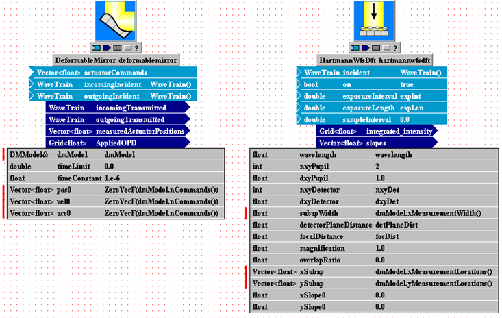
The AO configuration quantities that must be passed in are a collection of scalars, vectors and matrices stored in the final .mat file created during the AO configuration process. Perhaps the user is already acquainted with some WaveTrain procedures for reading vectors, arrays and grids from .mat files into system parameters, as explained in the WaveTrain User Guide (see mliLoad and related functions). Although the AO configuration quantities are simply more vectors and matrices, the WaveTrain editor interface uses additional specialized syntax and functions to read in the AO vectors and matrices.

(Parenthetically, we give a brief excuse for the convoluted syntax that follows. The procedure was originally developed because the AO configuration information can require much storage, and the use of C++ pointers ("*" variables) and references ("&" variables) avoids making copies of information such as OPD influence functions and reconstructor matrices.)

We now give the prescription for using the specialized syntax in the setting expressions. Let us first consider the DeformableMirror system, and the dmModel parameter, whose data type (see grey first column) is DMModel&.

Step 1:

(a) In the WaveTrain Runset Editor, create a run variable of Type TasatDMModel* (NOTE the trailing * in the Type name).
See the Runset Editor snippet below for an example.
(b) Assign the run variable Name: this is tdm in the example below, although the Name can be arbitrarily specified.
(c) In the Value field, enter the so-called constructor function, TasatDMModel(...). See below for the meaning of its arguments.

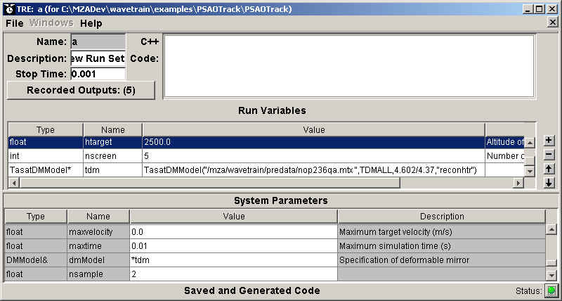
Step 2:

(a) In the WaveTrain System Editor, elevate the parameter of Type DMModel& from the DeformableMirror subsystem, so that it appears as a System Parameter in the Run Set Editor (as seen in the above picture).
(b) Assign the Value *tdm (NOTE the leading *), where tdm is whatever Name was assigned to the run variable in Step 1b.

(Step 2 can carried out before Step 1 in the model building)

The TasatDMModel(...) constructor function must have one of the following argument forms (items in bold type should be entered verbatim, items in italics are substituted with more specific information, and items in braces ({ }) are optional) :

TasatDMModel(filename, TDMALL)
TasatDMModel(filename, TDMALL, apscaling)
TasatDMModel(filename, TDMALL, apscaling, reconname)

where

filename is the name of the final .mat file created by the AO configuration process. This file must contain all the required geometry, OPD influence, and reconstructor data. The filename is a character variable that must be placed inside double quotes. In the filename spec, relative paths and the usual dot notations "./" and "../" are allowed. Note that forward slashes must be used as directory delimitors.

TDMALL is a flag which allows for additional flexibility not documented here.
The user should simply enter TDMALL exactly as written here.

apscaling is a scale factor to be applied to the size of the DM aperture as defined in the input file. Using the AO configuration tools, a configuration must be constructed for a particular aperture size. However, the same geometry may be useful on systems having a different aperture size. Setting apscaling to a value other than one causes the AO geometry defined in filename to be scaled by the specified factor. For example, suppose we devise an AO geometry using a 1.0 meter aperture. Later we can specify apscaling=0.75 to use the same influence function and reconstructor on a 0.75 meter system. When not specified, 1.0 is assumed.
CAUTION: When using apscaling ~= 1, one must careful about other setting expressions where one also extracts information from filename. One must extract the information in such a way that WaveTrain knows it is supposed to modify the value found in the file by the apscaling factor. In particular, this comment applies to the setting expressions in the HartmannWfsDft component for the parameters Dsub, xsub, and ysub. When apscaling=1, one might extract these parameters using an mliLoad(...) call (see the WaveTrain User Guide), but Wavetrain only knows to apply the apscaling factor if the quantities are extracted using a "method" of DMModel. The available "methods" are defined in the following subsection.

reconname Variable name of the desired reconstructor matrix contained in filename. Recall that files created by the AO configuration process can contain more than one reconstructor matrix. If reconname is not specified, the name is assumed to be "recon".

"Methods" of DMModel

In the case of the dmModel parameter in DeformableMirror, all available AO configuration information was passed in using the composite parameter called dmModel. On the other hand, the interface of HartmannWfsDft is arranged differently, and requires several specific items to be explicitly extracted from the AO configuration .mat file. The required items are:
(a) the locations of the centers of the subapertures (system parameters xSubap and ySubap, which were designated elsewhere in the present AO Guide as xsub and ysub)
(b) the subaperture width subapWidth.

There are two ways of extracting specific variables from the mass of AO configuration data, as needed by HartmannWfsDft (or potentially other WaveTrain components):
(1) Read required variables (e.g., xsub and ysub vectors) from the .mat file by using WaveTrain's file read functions, as explained in the WaveTrain User Guide (see the discussion of mliLoad(...) and related functions).
(2) Use "methods" associated with the "object" or "class" dmModel. This requires that a dmModel object, of data Type DMModel&, exist at the same system hierarchy level where we desire to use the "method". If this requirement is met, then xSubap, ySubap and subapWidth could be defined by the following setting expressions (which have been entered into the earlier System Editor screenshot of the HartmannWfsDft module):
   xSubap <--- dmModel.xMeasurementLocations()
   ySubap <--- dmModel.yMeasurementLocations()
   subapWidth <--- dmModel.xMeasurementWidth()

Notice that yet another "method" of dmModel was used to assign values to the parameters pos0, vel0, acc0 in DeformableMirror (see the earlier screen snapshot).

The following is a list of dmModel "methods" that users should find helpful:

Return Type	Call Syntax	Description
GridGeometry	OPDGrid()	Returns the GridGeometry of the OPD influence function.
int	nDOF()	Returns the number of degrees of freedom of the DM (usually the number of master actuators).
int	nCommands()	Returns the number of commands to be sent to the DM (usually the total number of commanded actuators, masters plus slaves).
int	nMeasurements()	Returns the number of measurements made by the WFS (twice the number of subapertures).
int	maxSubap1D()	Returns the maximal number of subapertures in either the x or y dimension.
Vector<float>	xMeasurementLocations()	Returns the x coordinates of the centers of the subapertures.
Vector<float>	yMeasurementLocations()	Returns the y coordinates of the centers of the subapertures.
float	xMeasurementSpacing()	Returns the spacing between centers of subapertures in the x direction.
float	yMeasurementSpacing()	Returns the spacing between centers of subapertures in the y direction.
float	xMeasurementWidth()	Returns the width of subapertures in the x direction.
float	yMeasurementWidth()	Returns the width of subapertures in the y direction.

Remaining parameter specifications

HartmannWfsDft In particular has numerous parameters in addition to the ones discussed above. These additional parameters must be set independently; i.e., their setting expressions cannot be read from information contained in the *.mat file generated by the AO configuration process. The general WaveTrain User Guide contains further information on WFS modeling, parameter definitions and setup.

Miscellaneous usage tips

WaveTrain allows for multiple adaptive optics geometries to be used within a single simulation run. This can be done by defining two run variables of type TasatDMModel*, named for example tdm1 and tdm2, and correspondingly flowing up two variables of type DMModel&, named for example dmModel1 and dmModel2. This would allow, e.g., two deformable mirrors to be used in a system, with completely different geometries and reconstructor information. (Previously, we have mentioned the possibility of running more than one AO system in a single simulation, with the same geometry but different reconstructors. That case does not require multiple run variables of type TasatDMModel* .)

.mat Interface File Contents

Output file of aogeom contains:

nact Total number of DM actuators.

nslav Number of slave actuators.

nmas Number of master actuators.
The number of inert actuators is ninert = nact - nslav - nmas. As discussed previously, the influence function and reconstructor calculations in the present release of the AO tools only work correctly for ninert = 0, i.e., for nslav+nmas = nact.

xact A column vector of dim (nact x1), containing the x-coordinates of the actuator locations. The actuator indexing convention has been described previously.

yact A column vector of dim (nact x1), containing the y-coordinates of the actuator locations.

actype A vector with length equal to nact. actype(i) determines whether the ith actuator is a master, slave, or an inert actuator. actype(i) = 1.0 if the ith actuator is a master actuator. actype(i) = -1.0 if the Ith actuator is a slave actuator. actype(i) = 0.0 if the Ith actuator is an inert actuator.

nmsmax The maximum number of master actuators that any slave actuator is slaved to.

idxmas A two-dimensional array which specifies which master actuators each slave responds to. The number of rows in idxmas is equal to nslav, the number of slave actuators, and the number of columns of idxmas is equal to nmsmax. The slave actuators are numbered from 1 to nslav in the same order as they appear in the numbering for all the actuators. If idxmas(i,1) = j, then the first master actuator (lowest numbered) that the ith slave actuator is slaved to is actuator number j. Actuator j must be a master actuator in this case. If a slave actuator is slaved to fewer than the maximum number of masters, the corresponding row of idxmas will contain some zeroes. For example, if the ith slave actuator is slaved to 2 masters and if nmsmax = 4, then idxmas(i,3) = idxmas(I, 4) = 0.

weight A two dimensional array of the same size as idxmas. The ith slave actuator will be given a voltage command which is a linear combination of the voltage commands sent to one or more masters. The locations of those masters is specified in idxmas. The coefficients in that linear combination are in the ith row of the array weight. Normally, the sum of the numbers in any row of weight would be unity. aoinf will fill the arrays idxmas and weight automatically using a very simple rule. If a slave actuator is adjacent to only one master, it is commanded with the same voltage as the master actuator. If it is adjacent to more than one master, it is commanded with the a weighted average of all the commands sent to the masters that it is adjacent to. The weights are proportional to the relative distance from the slave to each master.

nsub The number of WFS subapertures.

xsub A column vector of dim (nsub x1), containing the x-coordinates of the centers of the WFS subapertures. The subaperture indexing convention has been described previously.

ysub A column vector of dim (nsub x1), containing the y-coordinates of the centers of the WFS subapertures.

hs Subaperture center-center spacing. Recall that the x and y spacings of subaperture centers must be equal.

U This applies to Green's function influence functions only. A vector with length equal to nact. There are two parameters used in the clamped plate Green's function mirror model. One is the spring constant of the actuators, and the other relates the elongation of an actuator to the applied voltage. To determine these constants, an empirical influence function for the center actuator of an Itek mirror was used. The influence function was measured with 200 volts applied to the center actuator, all other actuators were not driven, and displacement of the mirror faceplate was recorded. The vector U contains the voltage commands for that test. It has zero entires for all except the center actuator which has 200 volts.

W This applies to Green's function influence functions only. A vector containing the displacements of all the actuators when 200 volts were applied to the middle actuator, based on the Itek data. The displacement of the middle actuator is 3.3 micrometers, the displacement of the nearest neighbor actuators is 5% of the displacement of center actuator, and the displacement of neighboring actuators separated along a diagonal from the center actuator is 1% of the center actuator displacement. The vectors U and W are hardwired in aoinf.

rc This applies to Green's function influence functions only. The radius at which the circular plate is assumed to be clamped in the Green's function model of the DM.

ninfl This applies to Green's function influence functions only. This parameter specifies the region over which the localized DM influence functions are computed. ninfl is set by changing the Green's function Actuator Influence Reach in aogeom. The influence of an actuator is only calculated out to ninfl actuator spacings and is assumed to be negligible beyond that distance.

nsi Number of intervals used in the Simpson's rule quadrature along each side of a subaperture to compute G-tilts induced by the DM. The user can modify this be changing the parameter # of Integ. Steps/Side of Subap.

rmas Radius of the master actuator circle.

rslav Radius of the slave actuator circle.

ract Radius of the circle containing all the actuators.

rsub Radius of the circle containing all the subapertures.

Output file of aoinf contains:

All of the above, plus:

opdif OPD influence function matrix, denoted A in the background discussion. When stored in a sparse format, as it appears in the Matlab workspace, opdif is a 2D array with dims (nx_reach * ny_reach) x n_act, where n{x,y}_reach is the number of OPD mesh points that correspond to the influence function reach (the reach was determined by the aogeom setup specifications).

mvtov A matrix that transforms a vector of voltage commands applied to the master actuators to voltage commands to all the actuators. The (row, col) dimensions of mvtov are (n_actx n_mas).

vtod A matrix that transforms a vector of voltages at all the actuators to displacements at all the actuators. The (row, col) dimensions of vtod are (n_actx n_act). As discussed previously, vtod is by default the unit matrix.

dtos A matrix that transforms all actuator displacements to all WFS subaperture slopes induced by the DM on the sensed wavefront. This is the DM slope influence matrix discussed in the background section, where it was designated S and defined by the relation s = S dd_act . The (row, col) dimensions of dtos are (2n_subx n_act).

mvtos A matrix that transforms a vector of voltages applied to the master actuators to all WFS subaperture slopes. The (row, col) dimensions of mvtos are (2n_subx n_mas). mvtos is equal to the matrix product dtos*vtod*mvtov. As discussed previously, and as shown in a Matlab terminal session, the composite mvtos is usually the only one of these four matrices that the user needs to deal with explicitly.

Save file generated after execution of aorecon should contain:

All of the above, plus:

recon1, {recon2, ...} Any number of reconstructor matrices. The particular matrix to be used by any given subsystem in a WaveTrain system will be specified as an argument in the TasatDMModel function. Unlike all the previously defined file variables, the actual names of recon1, {recon2, ...} are user-specified, as output argument names of the aorecon routine or its analogs.

Utility m-Files for Visualizing AO Quantities

Above, we have discussed the main computational routines that comprise the WaveTrain AO configuration tools. In addition to these, the AO toolset contains several utility routines that are helpful in visualizing AO variables. The utility routines are also Matlab m-files. The following list identifies and describes several such utility routines. A key purpose of the utility routines is to manipulate and plot 2D AO data that is stored in specialized 1D formats. As discussed elsewhere in this Guide, the 1D formats are the most practical method for storing data for generalized AO geometries.

actmap

Suppose we have any triple of 1D column vectors {F,x,y}, where vectors x and y contain a paired set of coordinates (x(i),y(i)), and where F(i) is the value of a scalar field at (x(i),y(i)).
Two typical AO examples are:
(1) {F,x,y} = {x-tilts or y-tilts at the subap centers, x-coords of subap centers, y-coords of subap centers};
(2) {F,x,y} = {surface displacements (opds) at actuators, x-coords of actuators, y-coords of actuators}.
In any such example, we often wish to make an image or mesh plot of the F data, using for example Matlab's imagesc function. But, to use imagesc or related display commands, we must rearrange the F vector into a 2D array with its elements in the correct spatial layout. actmap performs this rearrangement.

The Matlab calling syntax is:

>> F2D = actmap(F, x, y, {bval}, {reltol}, {padact});

where

F, x, y = three vectors of equal length, as described above.

bval = optional argument: value to assign to F2D at indices where no F data exists (default is NaN).

reltol = optional argument: not needed by user.

padact = optional argument: integer dimension of padding band to be added outside the support of F (default is 0).

F2D = 2D array containing the F values in the proper spatial layout. A typical use of F2D would be to serve as the input matrix to Matlab's imagesc plot function.

Note 1: To specify a later optional argument while defaulting a former, specify the empty matrix [ ] for the input argument to be defaulted.

Note 2: in the case of slope fields, another useful type of plot is the vector field plot, or "quiver" plot as it is called in Matlab. For example, to plot a slope field with the Matlab "quiver" function, only the 1D input vectors discussed above are required.

dmmap

Suppose we have a DM opd influence matrix computed using aoinf, and we also have a 1D vector of actuator displacements dact, which act at positions specified by the 1D coordinate vectors xact and yact. The dact may be actual displacement commands obtained from a WaveTrain simulation, or just an arbitrary set of test values constructed by the user. We may wish to make an image or mesh plot of the resulting DM displacement on the full influence function mesh (the "DM opd mesh"). As discussed previously, the DM opd mesh may be considerably denser than the dact mesh. In terms of notation introduced previously, what we want to do amounts to first computing the matrix product d_srf = Ad_act, and then converting the 1D d_srf to a 2D format suitable for input to a Matlab plot routine like imagesc. The function dmmap carries out these operations. dmmap requires the preliminary use of two other utility routines, opdc and actind.

The Matlab calling syntax is:

>> opd = dmmap(ixact, iyact, xopd, yopd, opdif, dact);

where

ixact, iyact = influence function actuator indices

xopd, yopd = opd mesh coordinates

To compute xopd, yopd, ixact, and iyact, use the helper routines actind and opdc as follows:
>> xopd = opdc(nxopd, dxopd); %nxopd, dxopd = dimension, spacing(m) of full DM opd mesh
%(see aoinf for discussion).
>> yopd = opdc(nyopd, dyopd); %aoinf only allows nyopd=nxopd, dyopd=dxopd
>> ixact = actind(xact, xopd);
>> iyact = actind(yact, yopd);

opdif = DM opd influence function matrix computed and saved by aoinf

dact = 1D vector of actuator displacements, acting at the xact, yact positions.
CAUTION: a complication may arise if slave actuators exist. Part of dmmap's action is to multiply opdif times the dact vector: to have the required length, dact must include all the actuators (master and slave). Depending on its source, a given dact may include only the masters (e.g., if dact comes from recording of WaveTrain simulated actuator commands). Therefore, depending on the source of dact, it may be necessary to first compute a modified dact via the multiplication dact_all = mvtov * dact_master. Then, dact_all is the quantity that must be entered into the dact input slot of dmmap.

opd = 2D array containing the DM displacements on the full opd mesh. The format of opd is suitable to serve as the input matrix to Matlab's imagesc or related plot functions.

Working with Asymmetric and/or Misregistered Systems

This capability will be provided in a future release of the AO tools.

If you need the capability at present for custom work, please contact MZA.